Hidden Markov Model

A Hidden Markov Model is a Bayes Network with these assumptions:
• Y_t depends only on Y_t-1
• X_t depends only on Y_t

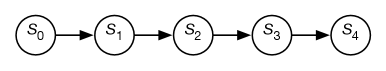
The belief network conveys the independence assumption:
$$
for\ all\ i \geq 0, P(S_{i+1}|S_i) = P (S_1|S_0)
$$

$$
P(S_i = s) = \sum_{s’} P(S_{i+1} = s \mid S_i = s’) * P(S_i = s’)
$$

In the context of the equation you’re referring to, $ s $ and $ s’ $ represent states in a Markov chain. Typically, $ s $ is used to denote the current state, while $ s’ $ (read as “s prime”) denotes a subsequent or different state that the system can transition into from the current state $ s $.

The summation over $ s’ $ in the equation indicates that you’re summing over all possible subsequent states that the system can transition to from the current state $ s $. This is part of the definition of a stationary distribution for a Markov chain, where the probability of being in any given state $ s $ is equal to the sum of the probabilities of transitioning to state $ s $ from all possible previous states $ s’ $, weighted by the probability of being in state $ s’ $ at the previous time step.

Key advantage of a hidden Markov model: Polynomial-time complexity

• Suppose there are |y| different speech sounds in English, and the length of the utterance is d centiseconds (|y| ≈ 50, d ≈ 100)
• Without the HMM assumptions, to compute f(x)= argmaxP(y₁, … , y_d|x₁, … , x_d) requires a time complexity of
  O{|y|^d} ≈ 50¹⁰⁰
• With an HMM, each variable has only one parent, so inference is O{|y|^d} ≈ 50²
• The computationally efficient algorithm that we use to compute f(x)= argmaxP(y₁, … , y_d|x₁, … , x_d) is called the Viterbi algorithm, named after the electrical engineer who first applied it to error correction coding.

it works much better than bayes

Text generated by a naïve Bayes model (unigram model):

• Representing and speedily is an good apt or come can different natural here he the a in came the to of to expert gray come to furnishes the line message had be these…

Text generated by a HMM (bigram model):

• The head and in frontal attack on an English writer that the character of this point is therefore another for the letters that the time of who ever told the problem for an unexpected…

Applications of HMMs

• Speech recognition HMMs:
  • Observations are acoustic signals (continuous valued)
  • States are specific positions in specific words (so, tens of thousands)
• Machine translation HMMs:
  • Observations are words (tens of thousands)
  • States are cross-lingual alignments
• Robot tracking:
  • Observations are range readings (continuous)
  • States are positions on a map

Viterbi Algorithm

The Viterbi algorithm is a computationally efficient algorithm for computing the maximum a posteriori (MAP) state sequence
$$
f(x)= argmax_{y_1, … , y_d}P(y_1, … , y_d|x_1, … , x_d)
$$

Notation

• Initial State Probability:

  • $ \pi_i = P(Y_1 = i)$

• Transition Probability:

  • $a_{i,j} = P(Y_t=j| Y_{t-1} = i)$

• Observation Probabilities:

  • $b_j(x_t) = P(X_t = x_t|Y_t=j)$

• Node Probability: Probability of the best path until node $ j $ at time $ t $

$$
v_t(j) = \max_{y_1,…,y_{t-1}} P(Y_1 = y_1 ,…, Y_{t-1} = y_{t-1}, Y_t = j, X_0 = x_0, …, X_t = x_t)
$$

• Backpointer: which node precedes node $ j $ on the best path?

$$
\psi_t(j) = \arg\max_{y_{t-1}} \max_{y_1,…,y_{t-2}} P(Y_1 = y_1 ,…, Y_{t-1} = y_{t-1}, Y_t = j, X_0 = x_0, …, X_t = x_t)
$$

How HMM Worked

Initiation → Iteration → Termination → Back-Tracing

• Initiation
  $v_1(i) = \pi_ib_i(x_1)$
• Iteration
  $v_t(j) = max v_{t-1}(i)a_{i,j}b_j(x_t)$
• Termination
  $y_d = argmax v_d{i}$
• Back-Tracing
  $y_t = \psi_{t+1}(y_{t+1})$

Example Question

Richard Feynman is an AI. He cannot see the weather, but he can see whether or not his creator, Elspeth Dunsany, brings an umbrella to work. Let $ R_t $ denote the event “it is raining on day $ t $,” and let $ U_t $ denote the event “Dr. Dunsany brings her umbrella on day $ t $.” Dr. Dunsany is an absent-minded professor; she often brings her umbrella when it’s not raining, and often forgets her umbrella when it’s raining. Richard’s model of Dr. Dunsany’s behavior includes the parameter $ P(R_1 = T) = 0.5 $, and the parameters shown in the tables below. What is $ P(R_2 = F, U_1 = T, U_2 = T) $?

$ P(R_t = T | R_{t-1} = r_{t-1}) $	$ r_{t-1} = F $	$ r_{t-1} = T $
$ r_t = F $	0.4	0.1
$ r_t = T $	0.8	0.7

$P(U_t = T | R_t = r_t)$	$r_t = F$	$r_t = T$
$ r_{t-1} = F $	0.4	0.1
$ r_{t-1} = T $	0.8	0.7

• Initial State Probability:

  • $ P(R_1 = T) = 0.5 $

• Transition Probabilities:

  • $ P(R_t = T | R_{t-1} = F) = 0.8 $
  • $ P(R_t = T | R_{t-1} = T) = 0.7 $
  • $ P(R_t = F | R_{t-1} = F) = 0.4 $
  • $ P(R_t = F | R_{t-1} = T) = 0.1 $

• Observation Probabilities (Probability of Dr. Dunsany bringing her umbrella given the weather):

  • $ P(U_t = T | R_t = F) = 0.4 $ (Probability she brings an umbrella when it’s not raining)
  • $ P(U_t = T | R_t = T) = 0.1 $ (Probability she brings an umbrella when it is raining)

These probabilities define the initial state distribution, the transition dynamics, and the observation model of a system, which are essential components of probabilistic models like Hidden Markov Models (HMMs).

The scenario you’ve presented involves conditional probabilities and is a typical example used in Bayesian inference or probabilistic models. Given the information in the image, we can calculate the probability that Dr. Dunsany brings her umbrella on day 2 given that it’s not raining on day 2, but it was raining on day 1.

The information given includes:

1. The initial probability that it’s raining on day 1: $ P(R_1 = T) = 0.5 $
2. The conditional probabilities of bringing an umbrella given the weather:
   • $ P(R_t = T | R_{t-1} = r_{t-1}) $: The probability that Dr. Dunsany brings an umbrella on day $ t $ given the weather on day $ t-1 $.
   • $ P(U_t = T | R_t = r_t) $: The probability that Dr. Dunsany brings an umbrella on day $ t $ given the weather on day $ t $.

With the tables provided, we can calculate the probability that Dr. Dunsany brings her umbrella on day 2 given the conditions specified.

We can apply the law of total probability to consider all possible weather scenarios from the previous day. Here is the formula based on the total probability theorem:

$ P(R_2 = F, U_1 = T, U_2 = T) = \\
\sum_{r_{t-1} \in {T, F}} P(R_2 = F | R_1 = r_{t-1}) \cdot P(U_1 = T | R_1 = r_{t-1}) \cdot P(U_2 = T | R_2 = F)
$

We would then substitute the values from the tables into the formula to calculate the desired probability. Would you like to proceed with this calculation?