Multi-layer Neural Nets
From linear to nonlinear classifiers
- Linear classifier
- a linear classifier computes $f(x) = argmax\ Wx$
- The resulting classifier divides the x-space into Voronoi regions: convex regions with piece-wise linear boundaries
- Nonlinear classifier
- Not all classification problems have convex decision regions with PWL boundaries!
- Here’s an example problem in which class 0 (blue) includes values of x near [0.8,0]T, but it also includes some values of x near [0.4,0.9]T
- You can’t compute this function using: $f(x) = argmax\ Wx$
- The solution: Piece-wise linear functions
- Nonlinear classifiers, can be learned using piece-wise linear classification boundaries
- Nonlinear regression problems, can be learned using piece-wise linear regression
- In the limit, as the number of pieces goes to infinity, the approximation approaches the desired solution
Multi-layer network
 |
|---|
A piece-wise linear function $f(x)$ can be represented by a two-layer neural network. First, the hidden nodes compute:
$$
h_j(x) = \max(0, w_j^{(1)T} x + b_j^{(1)})
$$
Then for PWL regression, the output is a weighted sum of the hidden nodes:
$$
f(x) = w^{(2)T}x + b^{(2)}
$$
…while for PWL classification, the output is the softmax or argmax of such a sum:
$$
f(x) = \text{softmax}(0, W^{(2)T} x + b^{(2)})
$$
Training a two-layer network: Back-propagation
Multi-layer Neural Nets
https://karobben.github.io/2024/02/18/LearnNotes/ai-multilayer/


