A Beginner's Guide to scRNA-Seq Data Integration

Single-cell RNA sequencing (scRNA-seq) has revolutionized our understanding of cellular heterogeneity and function. However, integrating datasets, especially from different labs or experiments, can be challenging. In this guide, we’ll walk through the process of integrating scRNA-seq datasets using Seurat and provide tips for newcomers to the field.

Why Integrate scRNA-Seq Data?

Integrating multiple scRNA-seq datasets allows researchers to compare or combine data from different experiments, conditions, or labs. This is crucial when aiming to:

• Combine datasets to increase sample size.
• Compare conditions across different experiments.
• Mitigate batch effects arising from different experimental conditions.

The Seurat Integration Workflow

Seurat, a popular R package for scRNA-seq data analysis, provides a robust framework for data integration. Here’s a step-by-step guide:

Preprocessing

Before integration, preprocess each dataset separately. This includes:

• Filtering cells.
• Normalizing data.
• Identifying variable features.

library(Seurat)
#DefaultAssay(seurat_obj1) <- "RNA"
#DefaultAssay(seurat_obj2) <- "RNA"
seurat_obj1 <- NormalizeData(seurat_obj1)
seurat_obj2 <- NormalizeData(seurat_obj2)
seurat_obj1 <- FindVariableFeatures(seurat_obj1, selection.method = "vst", nfeatures = 2000)
seurat_obj2 <- FindVariableFeatures(seurat_obj2, selection.method = "vst", nfeatures = 2000)

Performing log-normalization
0%   10   20   30   40   50   60   70   80   90   100%
[----|----|----|----|----|----|----|----|----|----|
**************************************************|

Calculating gene variances
0%   10   20   30   40   50   60   70   80   90   100%
[----|----|----|----|----|----|----|----|----|----|
**************************************************|
Calculating feature variances of standardized and clipped values
0%   10   20   30   40   50   60   70   80   90   100%
[----|----|----|----|----|----|----|----|----|----|
**************************************************|

Why nfeatures = 2000

The nfeatures parameter, when set to 2000 in the context of Seurat functions like FindVariableFeatures, specifies that the function should identify the top 2,000 most variable genes in the dataset. These variable genes are often used in downstream analyses, such as PCA, because they capture significant biological and technical variability that can help differentiate cell populations.

The choice of 2000 as the number of variable features is somewhat arbitrary but has become a common default in many scRNA-seq workflows. Here’s why:

1. Historical Precedence: Early scRNA-seq datasets were smaller, and selecting the top 2,000 variable genes was found to be a good balance between computational efficiency and capturing meaningful biological variability.

2. Computational Efficiency: Using a subset of genes (like the top 2,000 variable genes) instead of the entire transcriptome makes downstream computations (like PCA, clustering, and UMAP/t-SNE embedding) faster and more memory-efficient.

3. Biological Relevance: Genes that are variably expressed across cells often represent key markers that can differentiate cell types or states. By focusing on these genes, one can often capture the major axes of variation in the data.

However, it’s essential to understand that 2000 is not a magic number, and depending on the specific dataset and research question, a different number might be more appropriate. Here are some considerations:

• Dataset Size: For larger datasets with more cells, you might benefit from selecting more than 2,000 variable genes. Conversely, for smaller datasets, a smaller number might suffice.

• Biological Question: If you’re interested in subtle subpopulations or rare cell types, you might need to consider more genes to capture this granularity.

• Exploration: It’s often beneficial to experiment with different numbers of variable features to see how it impacts downstream analyses. For instance, you can try 1,000, 2,000, 3,000, etc., and observe how it affects clustering or the resolution of cell populations in UMAP/t-SNE plots.

In summary, while nfeatures = 2000 is a commonly used default, it’s crucial to understand its implications and adjust it as needed based on the specifics of your dataset and research goals.

The method 'vst' refers to “Variance Stabilizing Transformation.” In the context of Seurat and scRNA-seq data analysis, the VST method is used to identify highly variable genes across single cells.

Here’s a brief overview of the VST method:

Variance Stabilizing Transformation (VST):

1. Purpose: The main goal of VST is to stabilize the variance across the mean of the data. In the context of gene expression data, this means making the variance of gene expression values more consistent across different expression levels.

2. Why It’s Important: In raw count data, the variance often increases with the mean. This means that highly expressed genes naturally have higher variability just due to the nature of the data. VST aims to correct for this, allowing for the identification of genes that are genuinely variable across cells, not just because of their expression level.

3. How It Works: Without diving too deep into the math, VST uses a transformation that makes the variance of the data approximately constant across different mean values. This transformation is data-driven and is estimated from the data itself.

4. Application in Seurat: In Seurat’s FindVariableFeatures function, when the method is set to 'vst', the function will use the VST approach to identify genes that are highly variable after accounting for the relationship between variance and mean expression.

5. Comparison to Other Methods: Another common method used in Seurat for identifying variable genes is 'mean.var.plot', which fits a loess curve to the relationship between variance and mean expression. The VST method is often more robust, especially for larger datasets, but it’s always a good idea to understand and consider the implications of the method you’re using.

In summary, the VST method in Seurat is a way to identify highly variable genes in a manner that accounts for and corrects the relationship between variance and mean expression. This helps in pinpointing genes that are genuinely variable across cells, which can be crucial for downstream analyses like clustering and dimensionality reduction.

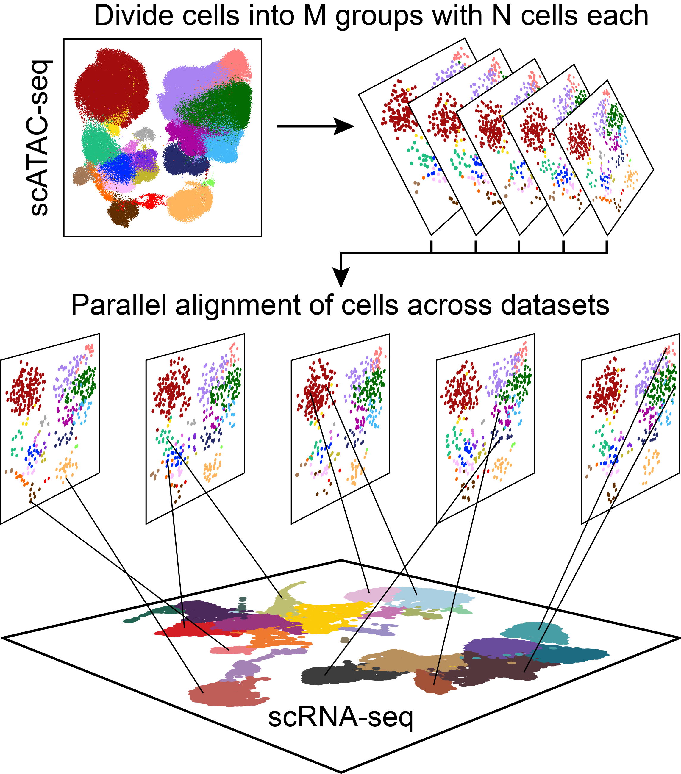
Identify Anchors

Seurat uses the concept of “anchors” to identify correspondences between cells in different datasets. These anchors are then used for data integration.

# FindIntegrationAnchors is really time consuming. Active per

anchor.features <- SelectIntegrationFeatures(object.list = list(seurat_obj1, seurat_obj2), nfeatures = 2000)
anchor.set <- FindIntegrationAnchors(object.list = list(seurat_obj1, seurat_obj2), anchor.features = anchor.features)

Scaling features for provided objects
  |++++++++++++++++++++++++++++++++++++++++++++++++++| 100% elapsed=11s  
Finding all pairwise anchors
  |                                                  | 0 % ~calculating  Running CCA
Merging objects
Finding neighborhoods
Finding anchors
Found 55971 anchors
Filtering anchors
Retained 18262 anchors
|++++++++++++++++++++++++++++++++++++++++++++++++++| 100% elapsed=04h 16m 22s

Integration

Seurat uses “anchors” to identify correspondences between cells in different datasets. These anchors are then used for data integration.

integrated.data <- IntegrateData(anchorset = anchor.set)
saveRDS(integrated.data, "integrated.rds")

Merging dataset 2 into 1
Extracting anchors for merged samples
Finding integration vectors
Finding integration vector weights
0%   10   20   30   40   50   60   70   80   90   100%
[----|----|----|----|----|----|----|----|----|----|
**************************************************|
Integrating data

Here, the integration steps are done. The following steps is for checking the integration quality and results.

Downstream Analysis

After integration, you can proceed with:

• Scaling the data.
• Running PCA.
• Clustering cells.
• Visualizing data using UMAP or t-SNE.

integrated.data <- ScaleData(integrated.data, verbose = FALSE)
integrated.data <- RunPCA(integrated.data, npcs = 30, verbose = FALSE)
integrated.data <- FindNeighbors(integrated.data, dims = 1:30)
integrated.data <- FindClusters(integrated.data, resolution = 0.5)
integrated.data <- RunUMAP(integrated.data, dims = 1:30)
DimPlot(integrated.data, group.by = "orig.ident")

3. Tips for Newbies in scRNA-Seq Integration

For those new to scRNA-seq integration, here are some essential tips:

• Quality Control: Ensure thorough QC on each dataset before and after integration.
• Visual Inspection: Use UMAP/t-SNE plots and heatmaps to visually inspect your data.
• Parameter Tuning: Adjust parameters based on your specific datasets.
• Biological Validation: Validate your findings with external data or experimental validation.
• Computational Considerations: Ensure you have enough memory and computational resources.
• Documentation: Keep detailed notes and consider using tools like R Markdown.
• Stay Updated: The field of scRNA-seq is rapidly evolving. Stay updated with the latest methods and best practices.
• Seek Feedback: Discuss your results with colleagues or experts in the field.

4. Conclusion

Integrating scRNA-seq datasets can be challenging, especially for newcomers. However, with the right tools, a systematic approach, and a focus on the underlying biology, it’s possible to derive meaningful insights from integrated datasets. As with all bioinformatics tasks, continuous learning and practice are key to mastering scRNA-seq data integration.

Errors

Error when running normalization:

NormalizeData(seurat_obj1)                                             

Performing log-normalization
0%   10   20   30   40   50   60   70   80   90   100%
[----|----|----|----|----|----|----|----|----|----|
**************************************************|
Error: Cannot add a different number of cells than already present

Solution:

seurat_obj1[["RNA"]] <- NormalizeData(seurat_obj1[["RNA"]])

duplicated cell-name

In CheckDuplicateCellNames(object.list = object.list) :
  Some cell names are duplicated across objects provided. Renaming to enforce unique cell names.

new.names1 <- paste0(colnames(seurat_obj1), "_P40")
seurat_obj1 <- RenameCells(object = seurat_obj1, new.names = new.names1)

# For seurat_obj2, add "_batch2" as a suffix
new.names2 <- paste0(colnames(seurat_obj2), "_P50")
seurat_obj2 <- RenameCells(object = seurat_obj2, new.names = new.names2)