Evaluating the quality of classification

Situation

I have a large, sparse dataset that I’ve analyzed using a neural network model borrowed from previous research. After classifying the data using this model, I applied dimensionality reduction, resulting in well-defined groups. To assess the quality of this classification, I’m considering evaluating the sparsity of classes in the reduced dimension space. One method I’m contemplating is examining the standard deviation in relation to the mean/median value for each group. Are there other effective methods to evaluate the classification based on the distribution in the reduced space?

How to start

Evaluating the quality of classification, especially in the context of redundancy and sparsity, can be a nuanced task. It sounds like you’re interested in understanding how well-separated or distinct the groups are after applying redundancy techniques on the classification results.

Here’s a structured approach to evaluate your classification results based on redundancy distribution:

1. Descriptive Statistics:

   • Mean/Median: Understand the central tendency of each group.
   • Standard Deviation (SD): Check the spread or variability within each group. A lower SD indicates that the data points are closer to the mean, suggesting tighter clusters or classes.
   • Skewness: Understand the symmetry of your distribution. Positive skewness indicates a long tail on the right, while negative skewness indicates a long tail on the left.
     • skewness(X)

2. Visualization:

   • Heatmaps: These can help you visualize the density and sparsity of your classes in the redundancy map.
   • Histograms/Box-plots: To visually inspect the distribution of each group.

3. Quantifying Sparsity:

   • Sparsity Ratio: It’s the ratio of the number of zero (or near-zero, depending on the threshold you set) elements to the total number of elements. A higher sparsity ratio indicates that the classes are more distinct in the redundancy map.
   • Gini Coefficient: Used in economics to measure inequality, it can also measure the inequality of the distribution of classes in a redundancy map. A Gini coefficient of 0 indicates perfect equality, while a Gini coefficient of 1 indicates maximum inequality.

4. Comparative Metrics:

   • Silhouette Score: Measures how close each sample in one cluster is to the samples in the neighboring clusters. Values range from -1 to 1, where a high value indicates that the object is well matched to its own cluster and poorly matched to neighboring clusters.
   • Davies-Bouldin Index: The lower the value, the better the clustering result. It evaluates intra-cluster similarity and inter-cluster differences.

5. Stability Analysis:

   • If possible, perform the same classification and redundancy process on different subsets of your data. If the results are consistent across different subsets, it adds to the validity of your analysis.

6. Ground Truth Comparison:

   • If there’s a “ground truth” or some external benchmark dataset that you can compare with, it can provide a clear evaluation of how well your classification aligns with known standards.

7. Entropy:

   • For each group or cluster, you can compute its entropy to gauge the randomness or unpredictability of its classification assignments. Lower entropy indicates that a cluster is predominantly made up of one class, whereas higher entropy indicates a mix of classes.

Lastly, remember that no single metric can fully capture the quality and nuances of your classification, especially in the context of redundancy and sparsity. Use a combination of metrics and visualizations to get a comprehensive view of the quality and then base your conclusions on the collective evidence.

Consider also cross-referencing your results with domain experts or literature in the field to ensure that your evaluations and conclusions align with the underlying phenomena you’re studying.

Skewness

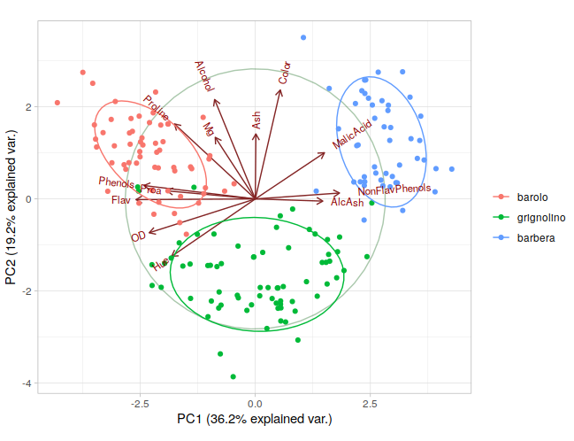
run PCA

We use the wine data as the example data. The classes information is in wine.class

## install ggbioplot
## remotes::install_github("vqv/ggbiplot")
## install.packages('plyr')
library(plyr)
library(ggbiplot)
library(ggplot2)
data(wine)
wine.pca <- prcomp(wine, scale. = TRUE)
## bioplot
ggbiplot(wine.pca, obs.scale = 1, var.scale = 1,
         groups = wine.class, ellipse = TRUE, circle = TRUE) +
  scale_color_discrete(name = '') +
  theme_light()+ theme(axis.title = element_text(size=10))

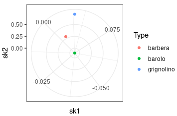
Check the Skewness

library(e1071) # for function skewness

score <- wine.pca
wine_types <- unique(wine.class)

skew_TB <- data.frame()
for(type in wine_types){
  subset_scores <- scores[wine.class == type, ]
  
  skewness_PC1 <- skewness(subset_scores[, 1])
  skewness_PC2 <- skewness(subset_scores[, 2])
  
  skew_TB <- rbind(skew_TB, data.frame(sk1 = skewness_PC1, sk2 = skewness_PC2, Type = type))
}

# visualization

ggplot(skew_TB, aes(sk1, sk2, color = Type)) + geom_point() + 
  theme_bw() + coord_polar(theta = 'x')

By polarizing the x-axis, the points closer to the center exhibit reduced skewness in both PC components, resulting in decreased sparsity.

Sparsity Ratio and Gini Coefficient

• Sparsity Ratio: To compute the sparsity ratio for the PCA scores, you’d typically set a threshold (e.g., a value close to 0) below which a score is considered as ‘sparse’ or ‘zero’. The sparsity ratio is then calculated as the number of scores below this threshold divided by the total number of scores.

• Gini Coefficient: This measures inequality among values. For the PCA scores, a Gini Coefficient close to 1 indicates high inequality (i.e., few scores dominate), whereas a value close to 0 indicates more equality among scores.

# following the code above

compute_sparsity_ratio <- function(data, threshold = 0.1){
  return(sum(abs(data) < threshold) / length(data))
}

SG_TB = data.frame()

for(type in wine_types){
  subset_scores_PC1 <- scores[wine.class == type, 1]
  subset_scores_PC2 <- scores[wine.class == type, 2]
  
  # Sparsity ratio for PC1 and PC2
  sparsity_PC1 <- compute_sparsity_ratio(subset_scores_PC1)
  sparsity_PC2 <- compute_sparsity_ratio(subset_scores_PC2)
  
  # Gini coefficient for PC1 and PC2
  gini_PC1 <- ineq::Gini(subset_scores_PC1)
  gini_PC2 <- ineq::Gini(subset_scores_PC2)

  SG_TB <- rbind(SG_TB, data.frame(Type = type, 
                                   index1 = c(sparsity_PC1, gini_PC1),
                                   index2 = c(sparsity_PC2, gini_PC2),
                                   index = c('Sparsity', "gigi")))
}