Negative Binomial Distribution | Introduction and examples

Negative Binomial Experiment

• The experiment consists of x repeated trials.
• Each trial can result in just two possible outcomes. We call one of these outcomes a success and the other, a failure.
• The probability of success, denoted by P, is the same on every trial.
• The trials are independent; that is, the outcome on one trial does not affect the outcome on other trials.
• The experiment continues until r successes are observed, where r is specified in advance.

Consider the following statistical experiment. You flip a coin repeatedly and count the number of times the coin lands on heads. You continue flipping the coin until it has landed 5 times on heads. This is a negative binomial experiment because:

• The experiment consists of repeated trials. We flip a coin repeatedly until it has landed 5 times on heads.
• Each trial can result in just two possible outcomes - heads or tails.
• The probability of success is constant - 0.5 on every trial.
• The trials are independent; that is, getting heads on one trial does not affect whether we get heads on other trials.
• The experiment continues until a fixed number of successes have occurred; in this case, 5 heads.
  Cite: Stat Trek^[1]

Geometric distribution is a special case of the negative binomial distribution.

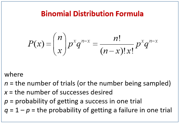
$$
b(x; r, P) = C_{x-1}^{r-1} \times P^r \times (1 - P)^{x - r}
$$

• $x$: The number of trials required to produce r successes in a negative binomial experiment.
• $r$: The number of successes in the negative binomial experiment.
• $P$: The probability of success on an individual trial.
• $Q$: The probability of failure on an individual trial. (This is equal to 1 - P.)
• $b(x; r, P)$: Negative binomial probability - the probability that an x-trial negative binomial experiment results in the rth success on the xth trial, when the probability of success on an individual trial is P.
• $C_n^r$: The number of combinations of n things, taken r at a time.

The Mean of the Negative Binomial Distribution

$μ = r / P$

• $μ$ is the mean number of trials
• $r$ is the number of successes
• $P$ is the probability of a success on any given trial.

Alternative Views of the Negative Binomial Distribution

$μ_ R = kP/Q$

• $R$: The negative binomial random variable
• $k$: the number of successes before the binomial experiment results in k failures

$μK = rQ/P$

• $K$: The negative binomial random variable
• $r$: the number of failures before the binomial experiment results in r successes

Geometric Distribution

The geometric distribution is a special case of the negative binomial distribution. It deals with the number of trials required for a single success. Thus, the geometric distribution is negative binomial distribution where the number of successes ® is equal to 1.
Cite: Stat Trek^[1:1]

$
b(x; r, P) = C_{x-1}^{r-1} \times P^r \times (1 - P)^{x - r}
$
$b(x; 1, P) = C_{x-1}^{0} \times P^1 \times (1 - P)^{x - 1}$
$b(x; 1, P) = P^1 (1 - P)^{x - 1}$
$b(x; 1, P) = P Q^{x - 1}$

Geometric Probability Formula. Suppose a negative binomial experiment consists of x trials and results in one success. If the probability of success on an individual trial is P, then the geometric probability is:

$$
g(x; P) = P Q^ {x - 1}
$$

Example

Bob is a high school basketball player. He is a 70% free throw shooter. That means his probability of making a free throw is 0.70. During the season, what is the probability that Bob makes his third free throw on his fifth shot?^[1:2]

From the example, we can know:
$P = 0.7$
$x = 4$
$r = 3$
So, we can have:
$b(5; 3, .7) = C_{4}^{2} \times P^3 \times (1 - P)^{5-3}$
$b(5; 3, .7) = C_{4}^{2} \times 0.7^3 \times 0.3^2$
$b(5; 3, .7) = 6 \times 0.7^3 \times 0.3^2 $
$b(5; 3, .7) = 18.522 % $

---

1. Stat Trek: Negative Binomial Distribution ↩︎ ↩︎ ↩︎