logistic regression in R

Logistic regression in R

Standard Logistic function for population growth

$$
P(m)= \frac{KP_{0}e^{rm}}{K + P_0(e^{rm} - 1)}
$$

• m: time point (x axis)
• r: α
• K: max

Test Data

reference: PriscillaBai 2018^[1]

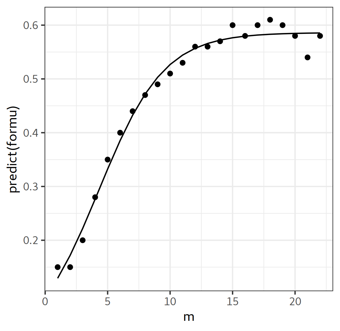
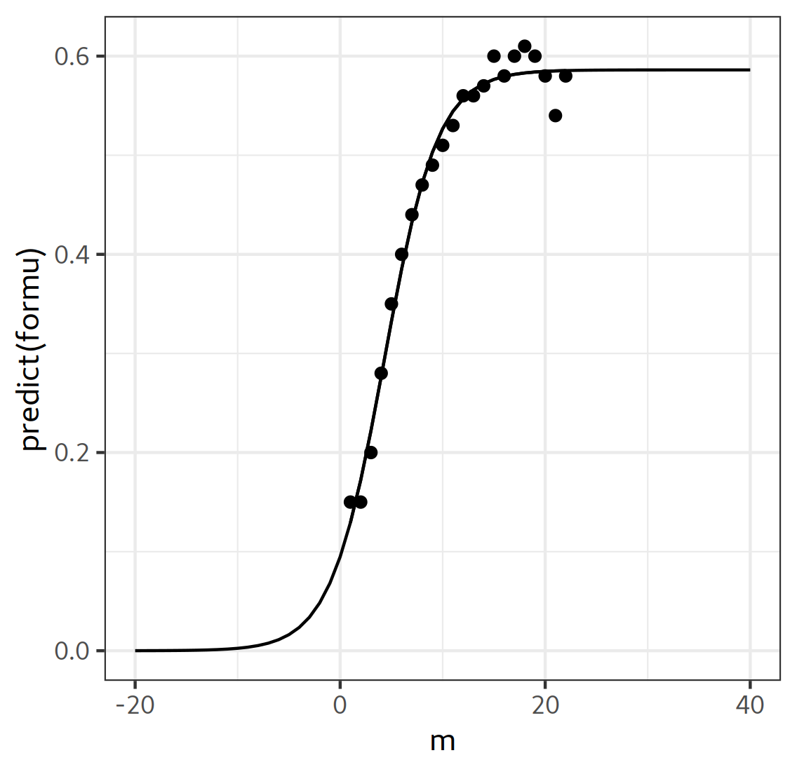
## Test Date set
n<-c(0.15,0.15,0.20,0.28,0.35,0.4,0.44,0.47,0.49,0.51,0.53,0.56,0.56,0.57,0.6,0.58,0.6,0.61,0.6, 0.58,0.54, 0.58)
m = c(1:length(n))
df<-as.data.frame(cbind(m,n))

## Regression

Regression

library(deSolve)

### 估计参数初始值| estimate
SS <- getInitial(n ~ SSlogis(m, alpha, xmid, scale), data = df)
K_start <- SS["alpha"]
R_start <- 1/SS["scale"]
P0_start <- SS["alpha"]/(exp(SS["xmid"]/SS["scale"])+1)

### 拟合函数方程
log_formula <- formula(n ~ K*P0*exp(R*m)/(K + P0*(exp(R*m) - 1)))
formu<-nls(log_formula, start = list(K = K_start, R = R_start, P0 = P0_start))

## Visualization
library(ggplot2)
ggplot() + geom_line(data=df,aes(m,predict(formu)))+
  geom_point(aes(x=m,y=n))+
  theme_bw()

plot more

We can check more information by:

formu

Nonlinear regression model
  model: n ~ K * P0 * exp(R * m)/(K + P0 * (exp(R * m) - 1))
   data: parent.frame()
 K.alpha  R.scale P0.alpha
 0.58610  0.38294  0.09482
 residual sum-of-squares: 0.006648

Number of iterations to convergence: 0
Achieved convergence tolerance: 1.708e-06

As a result, we can have the formula:

$$
P(m)= \frac{0.58610 * 0.09482 * e^{0.38294 * m}}{0.58610 + 0.09482(e^{0.38294 * m} - 1)}
$$

K <- SS["alpha"] # K = 0.58610
R <- 1/SS["scale"] # R = 0.38294
P0 <- SS["alpha"]/(exp(SS["xmid"]/SS["scale"])+1) # P0 = 0.09482

Log_r <- function(m){
   K * P0 * exp(R * m)/(K + P0 * (exp(R * m) - 1))
}

x=c(-20:40)
ggplot() + geom_line(data=df,aes(m,predict(formu)))+
  geom_point(aes(x=m,y=n))+
  theme_bw()+ geom_line(aes(x=x,y=Log_r(x)))

Slop calculation

$$
\frac{dP}{dm} = r×P(1-\frac{P}K)
$$

P = Log_r(SS['xmid'])
Slope = R_start[[1]] * P *( 1 - P/K_start[[1]])

ggplot() + geom_line(data=df,aes(m,predict(formu)))+
      geom_point(aes(x=m,y=n))+
      theme_bw()+ geom_line(aes(x=x,y=Log_r(x))) +  geom_abline(intercept = Log_r(SS["xmid"]) - SS["xmid"]*Slope, slope = Slope, color='steelblue', size =2, linetype=4)  + geom_point(aes(4.296, 0.293), color="salmon")   

Regression with binomial data

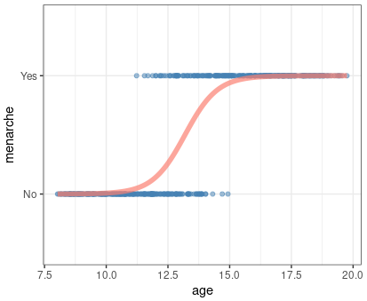
library(ISwR)
data(juul)
juul$menarche <- factor(juul$menarche, levels=c(1, 2), labels=c("No","Yes"))
juul$tanner <- factor(juul$tanner, levels=c(1:5))
juul.girl <- subset(juul, age>8 & age<20 & complete.cases(menarche))
# Note that this is a binomial data, we should use `binomial` arguments here
glm_menarche_age <- glm(menarche~age, family=binomial, data=juul.girl)
summary(glm_menarche_age)

Call:
glm(formula = menarche ~ age, family = binomial, data = juul.girl)

Deviance Residuals:
     Min        1Q    Median        3Q       Max  
-2.32759  -0.18998   0.01253   0.12132   2.45922  

Coefficients:
            Estimate Std. Error z value Pr(>|z|)    
(Intercept) -20.0132     2.0284  -9.867   <2e-16 ***
age           1.5173     0.1544   9.829   <2e-16 ***
---
Signif. codes:  0 ‘***’ 0.001 ‘**’ 0.01 ‘*’ 0.05 ‘.’ 0.1 ‘ ’ 1

(Dispersion parameter for binomial family taken to be 1)

    Null deviance: 719.39  on 518  degrees of freedom
Residual deviance: 200.66  on 517  degrees of freedom
AIC: 204.66

Number of Fisher Scoring iterations: 7

---

library(ggplot2)

X = juul.girl$age
Y = predict(glm_menarche_age, data.frame(age=X), type="resp")

# in the level, the "No" is 1, "Yes" is 2. So, we need to add 1 in the Y
ggplot(juul.girl, aes(x=age, y =menarche)) +
  geom_point(color="steelblue", alpha= .5) +
  geom_line(aes(x=X,y=Y+1), color="salmon", size=2, alpha = .7) +
  theme_bw()

© Karobben

library(deSolve)
TB <- read.csv("~/Downloads/df.csv")
TB2 <- TB[!is.na(TB$bloating_ratio),]
TB2 <- TB2[TB2$tumor!="Non-tumor",]
for(i in unique(TB2$genotype)){
    TMP <- TB2[TB2$genotype==i,]
}

n<- TMP$tumor_size
m = TMP$bloating_ratio
df<-as.data.frame(cbind(m,n))

model_mpg <- lm(formula = n ~ m, data = df)

Formula <- function(x){
  model_mpg$coefficients[[2]]*x+ model_mpg$coefficients[[1]]
}
ggplot() + geom_point(data=df, aes(m,n)) + geom_line(aes(x=x,y=Formula(x))) + theme_bw()






### 估计参数初始值| estimate
SS <- getInitial(n ~ SSlogis(m, alpha, xmid, scale), data = df)
K_start <- SS["alpha"]
R_start <- 1/SS["scale"]
P0_start <- SS["alpha"]/(exp(SS["xmid"]/SS["scale"])+1)

### 拟合函数方程
log_formula <- formula(n ~ K*P0*exp(R*m)/(K + P0*(exp(R*m) - 1)))
formu<-nls(log_formula, start = list(K = K_start, R = R_start, P0 = P0_start))

## Visualization
library(ggplot2)
ggplot() + geom_line(data=df,aes(m,predict(formu)))+
  geom_point(aes(x=m,y=n))+
  theme_bw()

---

1. PriscillaBai; R语言绘制逻辑斯蒂(logistic)生长曲线; 简书; 2018; Link ↩︎