GGplot | A tutorials for beginner

大量带图介绍: https://yutannihilation.github.io/allYourFigureAreBelongToUs/ggthemes/
扩展包介绍: http://www.ggplot2-exts.org

ggsave

ggsave(filename, plot = last_plot(), device = NULL, path = NULL, scale = 1, width = NA, height = NA, units = c("in", "cm", "mm"), dpi = 300, limitsize = TRUE, ...)
ggsave('plot.pdf', width=7,height=3)
ggsave('plot.png', width=400,height=300)

## 当pdf字体有问题时：
ggsave('test.pdf', width=7,height=3, device = cairo_pdf, family = "Song")

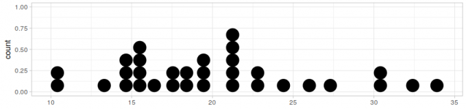
Dot plot

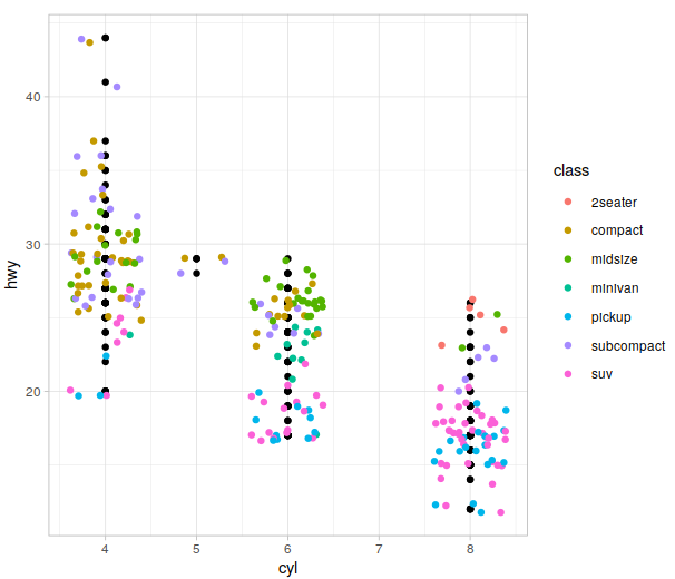
geom_point

ggplot(mpg) +geom_point(mapping =aes( x =displ, y =hwy, color =class))
ggplot(mpg) +geom_point(mapping =aes( x =V1, y =V2, color =V3, shape =V4, size=V5))

geom_dotplot

ggplot(mtcars, aes(x = mpg)) + geom_dotplot() + theme_light()

geom_jitter

ggplot(mpg, aes(cyl, hwy))+ geom_point() +geom_jitter(aes(colour = class))+ theme_light()

Line

geom_line & geom_path

library(ggplot2)
library(patchwork)

TB = data.frame(X=c(1,23,4,2,3,4,1,1,2,3,4,1,1,5,2,3),Y=c(1:16))

p1 <- ggplot(TB) + geom_line(aes(X,Y)) + labs(title='geom_line()')+ theme_light()
p2 <- ggplot(TB) + geom_path(aes(X,Y)) + labs(title='geom_patch()')+ theme_light()

geom_smooth

ggplot(data = mpg) + geom_point(mapping = aes(x = V1, y = V2)) + geom_smooth(mapping= aes(x=V1, y=V2))
######
## sting
ggplot(mpg , aes(x = displ, y = hwy)) + geom_point() +
  geom_smooth(method = "lm")

++geom_smooth(data=Growth_p,aes(x=ID,y=log(value+20)/3,group=ALL,color='OD Curve'),se = FALSE,span=0.75)

Extra Line

aux2 <- data.frame(cyl = c(4,6,8), x = c(2,3,4),y = c(10,10,10),
                   xend = c(2,3,4), yend = c(35,35,35),
                   x2 = c(3,4,5), xend2= c(3,4,5))
ggplot(mtcars, aes(x = drat)) +
  geom_line(aes(y = mpg, colour = "mpg")) +
  geom_line(aes(y = qsec, colour = "qsec")) +
  geom_segment(aes(x = x, y = y, xend = xend, yend = yend, colour = "xiaopang"),data= aux2, lty = 2) +
  geom_segment(aes(x = x2, y = y, xend = xend2, yend = yend, colour = "xiaomei"),data= aux2, lty = 2)

geom_boxplot

ggplot(box,aes(x=box$variable,y=box$value)) +geom_boxplot()

Bar

geom_bar

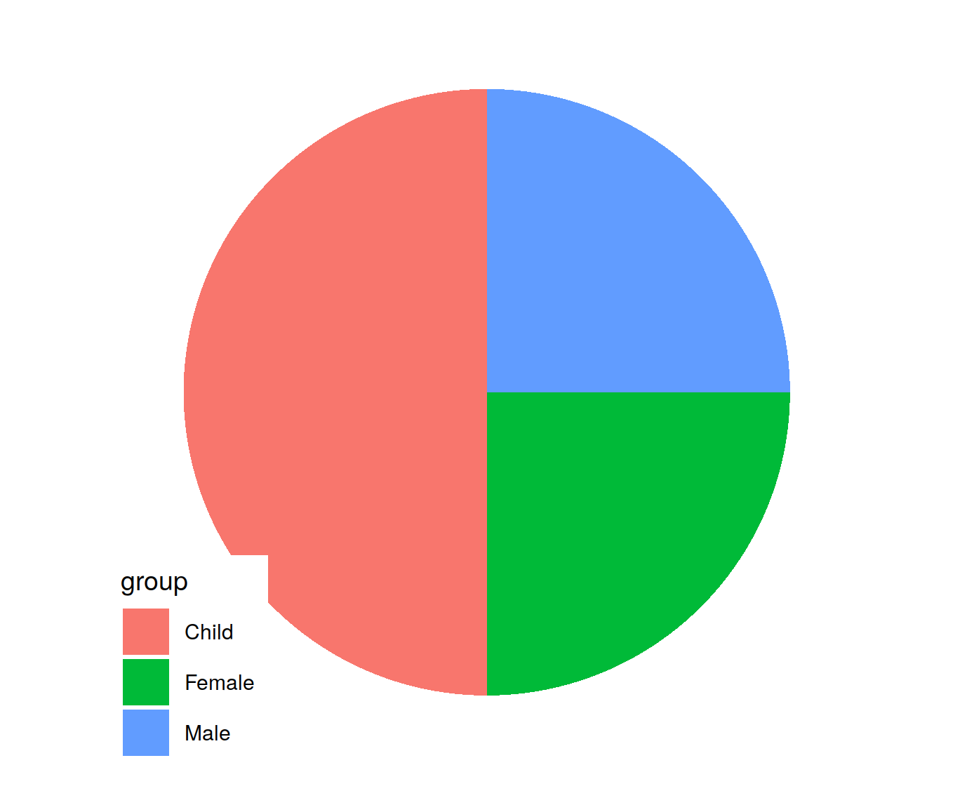
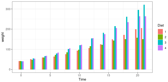
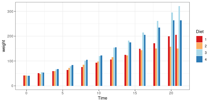
+ geom_bar(stat= 'identity')
### the number of the point
+ geom_bar(aes(fill=group),stat="identity")
### the mean of all point (stack togather)
+ geom_bar(aes(fill=group),stat="summary",fun.y="mean",position = 'stack')
### dont stact
+ geom_bar(aes(fill=group),stat="summary",fun.y="mean",position = 'dodge')

an easier way to draw bar plot

df <- data.frame(trt = c("a", "b", "c"), outcome = c(2.3, 1.9, 3.2))
ggplot(df, aes(trt, outcome)) + geom_col() + geom_point(color='red')

Position for bar

### Position
position = 'fill'
position = 'identity'
position = 'stack'
position = 'dodge'

More for Bar plot: Blog/语雀

from bar to pie

you just need adding + coord_polar("y", start=0) at the end of your code

More for pie: GitIO/语雀

Heatmap

ggplot(A, aes(x=Diet,y=A$Time)) + xlab("samples") + ylab(NULL) +
  theme_bw()+theme(panel.grid.major = element_blank()) +
  theme(legend.key=element_blank())+geom_tile(aes(fill=weight)) +
  scale_fill_gradient2(low="steelblue2",mid="white",high="red",midpoint =150)+
  scale_fill_gradient(low = "white", high = "red")

ggplot(A, aes(x=Diet,y=A$Time)) + xlab("samples") + ylab(NULL) +
  theme_bw()+
  theme(panel.grid.major = element_blank()) +
  theme(legend.key=element_blank())+
  geom_tile(aes(fill=weight)) +
  scale_fill_gradient2(low="steelblue2",mid="white",high="red",midpoint =150)+
  scale_fill_gradient(low = "white", high = "red")

Best theme for heatmap

## Best color for heatmap
library(RColorBrewer)
colorRampPalette(rev(brewer.pal(n = 7,name = "RdYlBu"))) -> cc
simplot(d) + scale_fill_gradientn(colors=cc(100)) + theme()

Fan plot

ggplot() + geom_bar() + coord_polar(theta = 'y')
## removing background
+theme(panel.grid=element_blank(),panel.border=element_blank(),axis.ticks=element_blank(),axis.text=element_blank(),axis.title=element_blank(),, panel.background = element_blank())
## or

library(ggthemes)
+theme_map()

geom_errorbar

+ geom_errorbar(aes(ymin=len-sd, ymax=len+sd),
 width=.2， position=position_dodge(.9))

Adding Equation

reference: weixin_43948357 2020

eq <- substitute(italic(y) == a + b %.% italic(x)~","~italic(R)^2~"="~r2~","~italic(P)~"="~p)
p + geom_text(aes(x = 4, y = 50, label = as.character(as.expression(eq))), parse = TRUE)

patchwork

library(patchwork)

p1 <- ggplot(mtcars,aes(mpg)) + geom_histogram() + theme_light() + ggtitle('histogram')
p2 <- ggplot(mtcars,aes(mpg)) + geom_freqpoly() + theme_light()  + ggtitle('freqpoly')

p2/p1

# order the legend
P11/P33 + plot_layout(guides = "collect")  & theme(legend.position = "right")

Axis

reference: 九茶 2015

+ scale_x_continuous(breaks=seq(0, 10, 5))
## 0: start
## 10: end
## 5: breaks

Switch Coordination

##switch X and Y
+ coord_flip()

Axis Limits

+ coord_cartesian(ylim = c(100,200), expand = F) # moving the panel
+ coord_fixed(ratio =2) #ratio = axis.y/axis.x
+ expand_limits(y=c(-12,18)) # similar like cartesian

Polar Axis

+ coord_polar(theta ="x", start = pi/3)
+ coord_polar(theta ="y", start = pi/3)

Scale Axis

## https://www.cnblogs.com/wkslearner/p/5635184.html
+scale_x_date(breaks=as.Date(c("2016-06-06","2016-06-13","2016-06-20","2016-06-27")),
              labels=c("06-06","06-13","06-20","06-27"),date_labels="%y/%m/%d")

Reverse axis

+ scale_x_reverse()
+ scale_y_reverse()

Legends

Basic usage:

+ theme( legend.position='none')

Position

legend.position = 'none'        # delete legend
legend.position = "left"        # Position left
legend.position = "right"       # Position right
legend.position = "bottom"      # Position bottom
legend.position = "top"         # Position Top
legend.position = c(0.9, 0.1)   # relative postion in right-bottom.

Legends’ name

# alter in the given scale
scale_color_gradient2(name = "My title")

# labs()
labs(color = "title for color",
     size  = "title for size",
     fill  = "title for fill")

Texts

labs

+ labs(title="MPO", x="Basket", y="U/g")
+ theme(plot.title = element_text(hjust = 0.5))

geom_text & geom_labels

library(ggrepel)
+geom_text_repel(aes(label=variable))
+geom_text(data=A,aes(x=V1,y=valuable,
            label=row.names(A4), colour =row.names(A4)),nudge_x = 0.5)

Annotate

annotate(geom, x = NULL, y = NULL, xmin = NULL, xmax = NULL,
  ymin = NULL, ymax = NULL, xend = NULL, yend = NULL, ...,
  na.rm = FALSE)
geom="text" |"rect"| "segment" | "pointrange"
 + annotate("segment", x = 2, xend = 4, y = 15, yend = 25, colour = "pink", size=3, alpha=0.6, arrow=arrow())

ggtitle

ggtitle("AAA")
theme(plot.title = element_text(hjust = 0.5))

Switch x labels (text.x)

## add the limits first and substitu...
+ scale_x_discrete(name ="Dose (mg)", limits=c(1:119),labels=as.character(A$X1))

Legends title

# alter in the given scale
scale_color_gradient2(name = "My title")

# labs()
labs(color = "title for color",
     size  = "title for size",
     fill  = "title for fill")

Facet

+ facet_grid(Group ~ .)
## Switch the side of the legen
+ facet_grid(Group ~ . switch = 'y')

## for GO enrichment
+ facet_grid(. ~ Cate,scales = "free_x",space = "free")
+ facet_wrap(~ V3, nrow = NULL, ncol = NULL, scales = "free")

Themes

Background

remove

+ theme(panel.grid.major =element_blank(),             #栅格线1
        panel.grid.minor = element_blank(),            #栅格线2
        panel.background = element_blank(),            #滑板底层
        axis.line = element_line(colour = "black"),    #轴线
        axis.ticks=element_blank(),                    #轴上点
        axis.text.y=element_blank(),                   #y文字
        axis.title.x =elemet_blank(),                  #y标题
        legend.position='none')                        #删标注

background color

panel.background = element_rect(fill = "lightblue",
                    colour = "lightblue",
                    size = 0.5, linetype = "solid"),

Levels

table$X=factor(table$X, levels=table[[1]])

theme()

+ theme(plot.title = element_text(hjust = 0.5),axis.text.x = element_text(angle = 45, hjust=1))

legend

##rm legend
+theme(legend.position='none')
##("none", "left", "right", "bottom", "top", or two-element numeric vect)

Colors (scale_fill/scale_color)

Default color palette for 4 samples:

library(ggplot2)
TB <- ChickWeight[ChickWeight$Chick %in% c(1,30, 40,50),]
summary(TB)

P <- ggplot(TB,aes(x=Time, y = weight, fill=Diet)) +
    geom_bar(stat = 'identity', position = 'dodge') + theme_bw()
P

    weight            Time           Chick    Diet  
Min.   : 41.00   Min.   : 0.00   1      :12   1:12  
1st Qu.: 66.75   1st Qu.: 5.50   30     :12   2:12  
Median :117.50   Median :11.00   40     :12   3:12  
Mean   :130.06   Mean   :10.92   50     :12   4:12  
3rd Qu.:172.00   3rd Qu.:16.50   18     : 0         
Max.   :321.00   Max.   :21.00   16     : 0         
                             (Other): 0         

If we have only few group like less than 13, we can use the preset color palette from RColorBrewer by scale_color_brewer

library("RColorBrewer")

#P + scale_color_brewer(palette =  "RdYlBu") # this is for line nad outline of the bar
P + scale_fill_brewer(palette =  "RdYlBu")

Palettes:
- Diverging
  BrBG, PiYG, PRGn, PuOr,
  RdBu, RdGy, RdYlBu, RdYlGn,
  Spectral

- Qualitative
  Accent, Dark2, Paired, Pastel1,
  Pastel2, Set1, Set2, Set3

- Sequential
  Blues, BuGn, BuPu, GnBu, Greens,
  Greys, Oranges, OrRd, PuBu, PuBuGn,
  PuRd, Purples, RdPu, Reds, YlGn,
  YlGnBu, YlOrBr, YlOrRd

If we only interesting in few of the color from the palette, we can print the color value and assign them with scale_color_manual/scale_fill_manual

Show the value of the colors:

brewer.pal(n = 12, name = "Paired")

'#A6CEE3''#1F78B4''#B2DF8A''#33A02C''#FB9A99''#E31A1C''#FDBF6F''#FF7F00''#CAB2D6''#6A3D9A''#FFFF99''#B15928'

##Example
scale_fill_manual(values=c("#FB882C","#5B88A0"))

If the group number is larger than 3 and we still want to using the color from palette, one resolution is combine multiple color palettes. Another Resolution is using colors from a palette or a list again and again.

library("RColorBrewer")

G_number = 100
N = 12
P + scale_fill_manual(values= head(rep(brewer.pal(n = N, name = "Paired"),round(G_number/N)+1), G_number))

library("ggthemes")

## Gradient
scale_fill_gradient() 允许分配一组双色连续渐变，low="white",high="red"
scale_fill_gradient2() 允许分配一组三色连续渐变，low="blue",mid="white",high="red"
## sed a group of colour
scale_fill_manual(values=c("Linen","Peru","PeachPuff","SandyBrown","Chocolate"))
## apply the Set on ggthemes
+ scale_colour_XXX()  # Tab to see more
+ scale_color_gradient(low = "cyan",high = "red")

scale_color_gradient(low = "cyan",high = "red")	scale_color_gradientn(values = seq(0,1,0.2),colours = c('cyan','blue','green','orange','red'))
© 天使不设防 2019	© 天使不设防 2019

More for plot

1. Cow plot

library(cowplot)
+ draw_plot(p1,0,0.5,0.5,0.5)+draw_plot(p2,0.5,0.5,0.5)
+draw_plot(pheat,0.5,0,0.5,0.5)
+draw_plot_label(c("A", "B"), c(0,0.5), c(1, 1), size = 20)
'''
Xl,Xr,Yt,Yzoom
draw_plot(p1,Xl,Yb,Xzoom,Yzoom,Pzoom)
'''

2. Patch Work

reference: 尘世中一个迷途小书僮

library(patchwork)
p1 <- ggplot() + ...
p2 <- ggplot() + ...
p1|p2

p1/p2

(p1|p2)|p2
GGlay = 'AA
##B'
p1 +p2 +plot_layout(design = GGlay)

3. Map

library(pacman)

rladies <- read_csv(url("https://raw.githubusercontent.com/d4tagirl/R-Ladies-growth-maps/master/rladies.csv"))%>% select(-1)

p_load(tidyverse, gganimate, maps, ggthemes)

ggplot()+borders("world", color="black", fill="steelblue4") +
                geom_point(data = rladies, aes(lon, lat, size=followers), color="firebrick3",
                alpha=0.6)+scale_size_continuous(range = c(2,8),
                breaks = c(250, 500, 750, 1000)) +
                labs(size="Followers", title="The development of R-Ladies'Twitter accounts",
                x=NULL,y=NULL)+theme(text = element_text(family = "Times New Roman",
                color = "deeppink"),plot.title = element_text(size=40,color = "#f9ba00"),
                plot.subtitle = element_text(size=14),axis.ticks = element_blank(),
                axis.text = element_blank(),panel.grid = element_blank(),
                panel.background = element_rect(fill="skyblue"),
                plot.background = element_rect(fill = "#333333"),
                legend.position = c(0.18,0.36),legend.background = element_blank(),
                legend.key = element_blank(),legend.text = element_text(size = 24),
                legend.title = element_text(size=28, color = "orangered3"))

More for maps, please go to see: GGplot Map

Extra

Details for theme

###########################
### Parameter of theme
###########################
line  #all line elements (element_line)
rect  #all rectangular elements (element_rect)
text  #all text elements (element_text)
title #all title elements: plot, axes, legends (element_text; inherits from text)
aspect.ratio  #aspect ratio of the panel
axis.title  #label of axes (element_text; inherits from text)
axis.title.x  #x axis label (element_text; inherits from axis.title)
axis.title.y  #y axis label (element_text; inherits from axis.title)
axis.tex  #tick labels along axes (element_text; inherits from text)
axis.text.x #x axis tick labels (element_text; inherits from axis.text)
axis.text.y #y axis tick labels (element_text; inherits from axis.text)
axis.ticks  #tick marks along axes (element_line; inherits from line)
axis.ticks.x  #x axis tick marks (element_line; inherits from axis.ticks)
axis.ticks.y  #y axis tick marks (element_line; inherits from axis.ticks)
axis.ticks.length #length of tick marks (unit)
axis.line #lines along axes (element_line; inherits from line)
axis.line.x #line along x axis (element_line; inherits from axis.line)
axis.line.y #line along y axis (element_line; inherits from axis.line)
legend.background #background of legend (element_rect; inherits from rect)
legend.margin #extra space added around legend (unit)
legend.key  #background underneath legend keys (element_rect; inherits from rect)
legend.key.size #size of legend keys (unit; inherits from legend.key.size)
legend.key.height #key background height (unit; inherits from legend.key.size)
legend.key.width  #key background width (unit; inherits from legend.key.size)
legend.text #legend item labels (element_text; inherits from text)
legend.text.align #alignment of legend labels (number from 0 (left) to 1 (right))
legend.title  #title of legend (element_text; inherits from title)
legend.title.align  #alignment of legend title (number from 0 (left) to 1 (right))
legend.position #the position of legends ("none", "left", "right", "bottom", "top", or two-element numeric vector)
legend.direction  #layout of items in legends ("horizontal" or "vertical")
legend.justification  #anchor point for positioning legend inside plot ("center" or two-element numeric vector)
legend.box  #arrangement of multiple legends ("horizontal" or "vertical")
legend.box.just #justification of each legend within the overall bounding box, when there are multiple legends ("top", "bottom", "left", or "right")
panel.background  #background of plotting area, drawn underneath plot (element_rect; inherits from rect)
panel.border  #border around plotting area, drawn on top of plot so that it covers tick marks and grid lines. This should be used with fill=NA(element_rect; inherits from rect)
panel.margin  #margin around facet panels (unit)
panel.margin.x  #horizontal margin around facet panels (unit; inherits from panel.margin)
panel.margin.y  #vertical margin around facet panels (unit; inherits from panel.margin)
panel.grid  #grid lines (element_line; inherits from line)
panel.grid.major  #major grid lines (element_line; inherits from panel.grid)
panel.grid.minor  #minor grid lines (element_line; inherits from panel.grid)
panel.grid.major.x  #vertical major grid lines (element_line; inherits from panel.grid.major)
panel.grid.major.y  #horizontal major grid lines (element_line; inherits from panel.grid.major)
panel.grid.minor.x  #vertical minor grid lines (element_line; inherits from panel.grid.minor)
panel.grid.minor.y  #horizontal minor grid lines (element_line; inherits from panel.grid.minor)
panel.ontop #option to place the panel (background, gridlines) over the data layers. Usually used with a transparent or blankpanel.background. (logical)
plot.background #background of the entire plot (element_rect; inherits from rect)
plot.title  #plot title (text appearance) (element_text; inherits from title)
plot.margin #margin around entire plot (unit with the sizes of the top, right, bottom, and left margins)
strip.background  #background of facet labels (element_rect; inherits from rect)
strip.text  #facet labels (element_text; inherits from text)
strip.text.x  #facet labels along horizontal direction (element_text; inherits from strip.text)
strip.text.y  #facet labels along vertical direction (element_text; inherits from strip.text)
strip.switch.pad.grid #space between strips and axes when strips are switched (unit)
strip.switch.pad.wrap #space between strips and axes when strips are switched (unit)

Details for element

margin(t = 0, r = 0, b = 0, l = 0, unit = "pt")
element_blank()
element_rect(fill = NULL, colour = NULL, size = NULL,
  linetype = NULL, color = NULL, inherit.blank = FALSE)
element_line(colour = NULL, size = NULL, linetype = NULL,
  lineend = NULL, color = NULL, arrow = NULL,
  inherit.blank = FALSE)
element_text(family = NULL, face = NULL, colour = NULL,
  size = NULL, hjust = NULL, vjust = NULL, angle = NULL,
  lineheight = NULL, color = NULL, margin = NULL, debug = NULL,
  inherit.blank = FALSE)
rel(x)