Random Forest

Basic Architectures

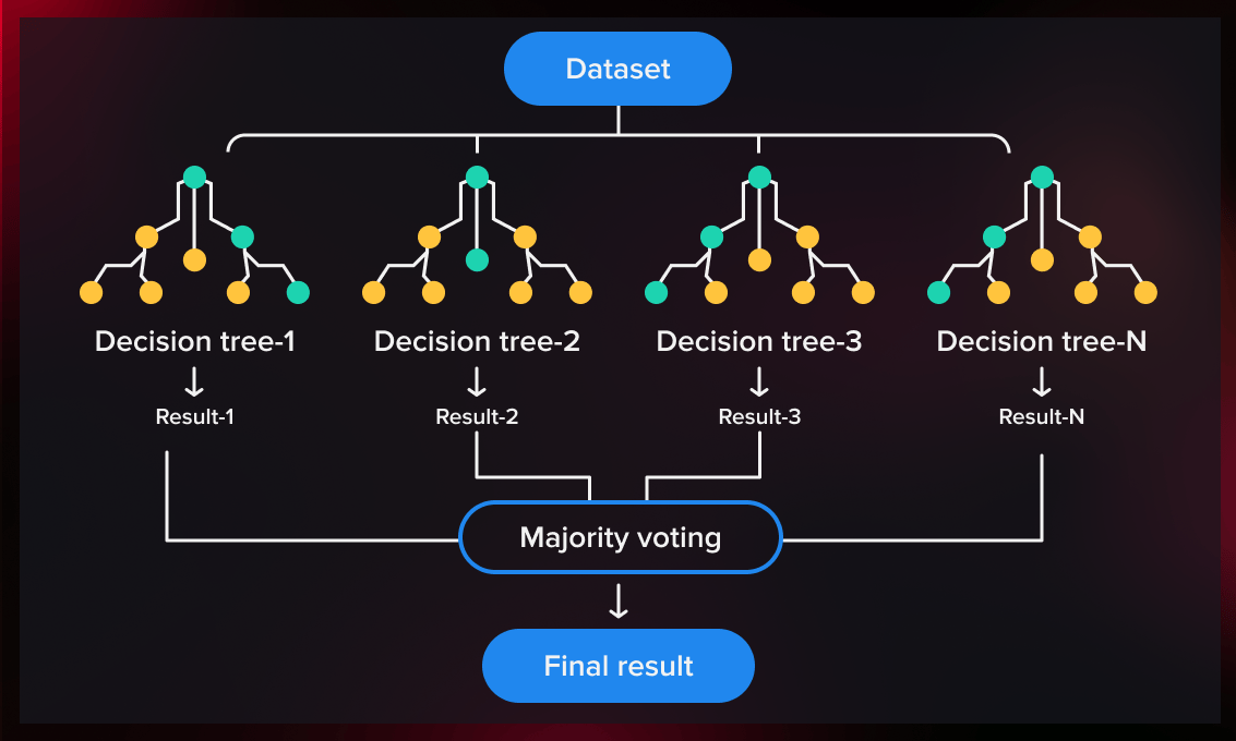
1. Bootstrap Sampling: Random subsets of the training data are created with replacement, known as bootstrap samples. Each subset is used to train an individual decision tree.
2. Feature Randomness: For each tree, a random subset of features is considered at each split, reducing correlation among trees and improving generalization.
3. Multiple Decision Trees: Multiple decision trees are grown independently using the bootstrap samples. Each tree makes a prediction for a given input.
4. Ensemble Output: For classification, the output is typically based on majority voting across all trees, while for regression, the final output is an average of all tree predictions.

Limitations

• Many different trees can lead to similar classifications
• The algorithm to build a decision tree grows each branch just deeply enough to perfectly classify the training examples
  • potential overfit
• Randomness in identification of splits: features, thresholds
  • better splits may have not been considered
• Addressed through Random Forests

Basic of Random Forest

Tree Expanding

Random forest is build on number of decision trees. For avoiding the overfit, early stop is needed during the tree expanding.

• It stop when
  • depth(branch_node) >= max_depth (manual)
  • size(dataset) <= min_leave_size (manual)
  • all elements in dataset in same class

Decision Making

The best decision made could be evaluate by the “entropy”.

1. 2 classes:
   Here are the formulas from the image converted into Markdown format:

• $ \text{Entropy}(S) = -P(A) \log_2 P(A) - P(B) \log_2 P(B) $
  • $ N = |A| + |B| $
  • $ P(A) = \frac{|A|}{N}, \quad P(B) = \frac{|B|}{N} $

2. C classes:

• $ \text{Entropy}(S) = - \sum_{i=1}^C P_i \log_2 P_i $
  • Each class $ i $ with probability $ P_i $.

Information Gain

Goal: The goal is to maximize Information Gain at each split, which corresponds to choosing features that result in subsets with the least entropy, making the data more pure (less mixed) after the split. In Random Forest and decision tree learning, the feature with the highest Information Gain is selected for splitting at each node.

• Definition: Information Gain measures the reduction in entropy (or uncertainty) after splitting a dataset. It helps to determine the best feature for splitting the data.
• Entropy Before Split: The initial dataset $ S $ has an entropy $ \text{Entropy}(S) $, which quantifies the impurity or randomness in the dataset.
• Entropy After Split: When the dataset is split into subsets $ S_l $ and $ S_r $, each subset has its own entropy: $ \text{Entropy}(S_l) $ and $ \text{Entropy}(S_r) $.
• Weighted Entropy: The weighted average of the entropy of the subsets after the split is given by:
  $$
  \text{Entropy}_{\text{after split}} = \frac{|S_l|}{|S|} \text{Entropy}(S_l) + \frac{|S_r|}{|S|} \text{Entropy}(S_r)
  $$
• Information Gain Calculation: The Information Gain for the feature $ x^{(i)} $ is calculated as the difference between the entropy before and after the split:
  $$
  \text{Information Gain} = \text{Entropy}(S) - \text{Entropy}_{\text{after split}}
  $$

The symbols $ |S| $, $ |S_l| $, and $ |S_r| $ represent the cardinalities or the sizes of the respective sets, meaning they indicate the number of elements in each set.

Missing Values

• In splits, if an item misses the feature value that decide where it goes
  • Estimate it based on other examples: mode or mean
• Consider only the examples in the corresponding branch

Decision Tree in Random Forest

For get the best “Decision” in each branch, iterating through all possible splits at each node can be computationally expensive, especially for large datasets and numerous features. However, decision trees (and Random Forests) use several optimization techniques to find the best split efficiently, while managing computational cost:

1. Feature and Threshold Selection Strategy

• Greedy Algorithm: Decision tree algorithms commonly use a greedy approach to split at each node. They do not explore all possible trees but instead make the locally optimal choice (the split that maximizes Information Gain or minimizes entropy) at each step. While this doesn’t guarantee a globally optimal tree, it is computationally efficient.
• Threshold Optimization: Rather than testing every possible threshold for each feature, the algorithm often considers a subset of thresholds. If the feature is numeric, thresholds are typically evaluated at points between consecutive, sorted feature values.

2. Random Forest Feature Subsampling

• In Random Forests, at each node, only a random subset of features is considered for splitting, rather than evaluating all features. This greatly reduces the number of calculations needed, enhances computational efficiency, and decorrelates the trees in the ensemble (increasing robustness).

3. Heuristics to Reduce Computation

• Best First Split: During the process, the split that gives the maximum Information Gain is stored, and the search for a better split continues until the end of the subset of considered thresholds. If no better split is found, the stored one is selected.
• Stopping Conditions: To further reduce resource usage, decision tree growth is often constrained by stopping criteria such as maximum depth, minimum number of samples per leaf, or if a split provides insufficient improvement.

4. Approximations for Efficiency

• Bin-based Thresholds: For numerical features, rather than considering every possible value as a split point, values can be grouped into bins. The potential split thresholds are then defined based on these bins.
• Pre-sorting Features: In some implementations, features are pre-sorted, so determining potential split points for numeric features can be faster.

5. Iterative Splitting and Best Split Finding

• For categorical features, the split can be done in subsets if there are many categories, or by considering binary splits. For numerical features, it evaluates splits between values.
• Yes, it does involve iteration, but the optimizations listed above ensure that this iteration is performed in a manageable and efficient way without explicitly iterating through every possible split for all features.

Balancing Efficiency and Quality of Decision Trees

The combination of the above techniques allows decision trees to strike a balance between:

1. Finding Good Splits: Even if the splits aren’t absolutely perfect, they are often good enough to form a strong decision tree.
2. Limiting Resource Waste: Efficient search heuristics and optimizations are used to reduce the exhaustive computational cost.

In Random Forest:

1. Choose $ m = \sqrt{|x|} $ Features at Random
   • Instead of evaluating all features for a potential split, a random subset of features is selected to reduce computation. The number of features selected ($ m $) is proportional to the square root of the total number of features ($ |x| $).
   • This is a common technique in Random Forests to decorrelate individual decision trees and make the algorithm computationally efficient. It prevents overfitting by introducing randomness and limits the number of features under consideration at each node.
2. Identify Candidate Splits for the Selected Feature $ x^{(i)} $
   • Feature Sorting:
     • The feature values ($ x^{(i)} $) can be sorted to determine the best thresholds for splitting the dataset.
   • Class Boundaries as Thresholds:
     • The sorted feature values are evaluated to find boundaries between different classes.
   • Sort Data Items According to Feature Value:
     • All data points are sorted by their value for the feature $ x^{(i)} $. This allows easy identification of candidate split points.
   • Adjacent Pairs in Different Classes:
     • The algorithm looks for adjacent pairs of data points where one belongs to a different class than the other. This suggests a potential decision boundary.
     • These pairs, $ (item_0, item_1) $, are identified since they may represent a significant change in class, making them good candidates for splitting.
   • Threshold Midway Between $ item_0 $ and $ item_1 $:
     • The threshold for the split is placed midway between these adjacent items from different classes. This ensures that the split captures the difference between the classes as effectively as possible.
3. Randomly Select $ k $ Thresholds
   • To further limit the number of potential splits to evaluate, the algorithm randomly selects $ k $ thresholds from the identified candidate thresholds. This further reduces computational cost while maintaining a good chance of finding an effective split.
   • This random sampling balances computational efficiency with the quality of the splits, ensuring that the decision tree doesn’t become too computationally expensive.
4. Summary
   The image explains a process that helps reduce the number of potential splits evaluated at each node:
   1. Random Subset of Features: Only a random $ m $ features are considered.
   2. Identifying Thresholds: For each selected feature, potential split thresholds are identified by analyzing class boundaries.
   3. Random Selection of Split Points: A random subset of the identified thresholds is evaluated.
      These steps are taken to avoid an exhaustive search, reduce computational resources, and prevent overfitting, particularly in Random Forests where multiple trees are built.

Step-by-Step Explanation with Equations and Code

Step 1: Choosing $ m = \sqrt{|x|} $ Features at Random

• Suppose you have $ |x| $ features in your dataset.
• To decide the split, randomly select $ m $ features to evaluate, where:
  $$
  m = \sqrt{|x|}
  $$

Python Code Representation:

import numpy as np

# data from: https://www.kaggle.com/datasets/uciml/pima-indians-diabetes-database?resource=download

import pandas as pd

data = pd.read_csv('/home/yiran/Downloads/diabetes.csv')
features = d.columns[:-1]

# Total number of features
num_features = len(features)

# Choose m features at random
m = int(np.sqrt(num_features))
selected_features = np.random.choice(features, m, replace=False)

Step 2: Identify Candidate Splits for a Feature $ x^{(i)} $

For each feature selected, you need to determine possible thresholds to split the data.

Steps in Code:

1. Sort Feature Values:

   • For the selected feature $ x^{(i)} $, sort the data points by their feature values.

2. Identify Boundaries Between Classes:

   • Find the pairs of data points that belong to different classes.
   • Calculate candidate thresholds midway between these pairs.

Equations for Finding Thresholds:

• Let $ x^{(i)}_j $ represent the feature value for data point $ j $.

• Sort all values of feature $ x^{(i)} $:
  $$
  x^{(i)}_1, x^{(i)}_2, \ldots, x^{(i)}_n \quad \text{where } x^{(i)}_1 < x^{(i)}_2 < \ldots < x^{(i)}_n
  $$

• Identify the adjacent pairs that belong to different classes. For a pair of adjacent items $ (x^ {(i)}_ j, x^ {(i)}_ {j+1}) $ from different classes, the candidate threshold $ t_j $ is given by:
  $$
  t_ j = \frac{x^ {(i)}_ j + x^ {(i)}_ {j+1}}{2}
  $$

Python Code Representation:

# Assume we have a data structure `data` which contains features and labels
# We are focusing on the selected feature xi

data = TB.T.to_dict()
data = [data[i] for i in data]

for feature in selected_features:
    # Sort data based on the selected feature's value
    sorted_data = sorted(data, key=lambda d: d[feature])
    # Find candidate thresholds
    candidate_thresholds = []
    for j in range(len(sorted_data) - 1):
        # If the class label changes between adjacent items
        if sorted_data[j]['Outcome'] != sorted_data[j + 1]['Outcome']:
            # Find the midpoint between two adjacent feature values
            threshold = (sorted_data[j][feature] + sorted_data[j + 1][feature]) / 2
            candidate_thresholds.append(threshold)

note

In the code sorted_data = sorted(data, key=lambda d: d[feature])

feature_value_pairs = [(d, d[feature]) for d in data]
# Step 2: Sort based on the feature value
feature_value_pairs_sorted = sorted(feature_value_pairs, key=lambda pair: pair[1])
# Step 3: Extract the sorted data points
sorted_data = [pair[0] for pair in feature_value_pairs_sorted]

Step 3: Randomly Select $ k $ Thresholds

• Randomly pick $ k $ thresholds from the candidate thresholds identified in the previous step to reduce computation.

Equation:

• Suppose $ T = { t_1, t_2, \ldots, t_p } $ is the set of candidate thresholds.
• Select $ k $ thresholds randomly from $ T $:
  $$
  T_{\text{selected}} = { t_{i_1}, t_{i_2}, \ldots, t_{i_k} }, \quad \text{where } i_j \in {1, \ldots, p}
  $$

Python Code Representation:

some_predefined_k = 15
# Number of thresholds to randomly select
k = min(len(candidate_thresholds), some_predefined_k)

# Randomly select k thresholds from candidate_thresholds
selected_thresholds = np.random.choice(candidate_thresholds, k, replace=False)

Step 4: Compute Information Gain for Each Split

• Iterate through the selected thresholds to compute the Information Gain and select the best one.

Equation for Information Gain:

• For a given threshold $ t $, split the data into two subsets:
  $$
  S_l = { x \in S : x^{(i)} \le t }, \quad S_r = { x \in S : x^{(i)} > t }
  $$

• Compute the weighted entropy after the split:
  $$
  \text{Entropy}_{\text{after}} = \frac{|S_l|}{|S|}\text{Entropy}(S_l) + \frac{|S_r|}{|S|}\text{Entropy}(S_r)
  $$

• Compute the Information Gain:
  $$
  \text{Information Gain} = \text{Entropy}(S) - \text{Entropy}_{\text{after}}
  $$

Python Code Representation:

def entropy(data):
    # Assume `data` has a function to calculate entropy
    labels = [d['Outcome'] for d in data]
    # Count the occurrences of each label
    label_counts = Counter(labels)
    total_count = len(data)
    # Calculate the entropy
    ent = 0
    for count in label_counts.values():
        # Calculate the probability of each label
        p = count / total_count
        # Add to entropy, using the formula -p * log2(p)
        if p > 0:
            ent -= p * np.log2(p)
    return ent

best_gain = -np.inf
best_threshold = None

for threshold in selected_thresholds:
    # Split the data into left and right based on the threshold
    left_split = [d for d in sorted_data if d[feature] <= threshold]
    right_split = [d for d in sorted_data if d[feature] > threshold]
    
    # Calculate the weighted entropy of the two subsets
    p_left = len(left_split) / len(sorted_data)
    p_right = len(right_split) / len(sorted_data)
    
    entropy_after = p_left * entropy(left_split) + p_right * entropy(right_split)
    gain = entropy(sorted_data) - entropy_after
    
    # Update the best gain and threshold
    if gain > best_gain:
        best_gain = gain
        best_threshold = threshold

Summary

1. Select Features Randomly: $ m = \sqrt{|x|} $ features are selected randomly to evaluate.
2. Determine Candidate Thresholds: For each feature, the data is sorted, and class boundaries are used to identify potential split points.
3. Random Threshold Selection: From the candidate thresholds, a random subset is chosen to reduce computational cost.
4. Calculate Information Gain: Evaluate the Information Gain for each threshold to find the best split.

These steps ensure that the decision tree algorithm efficiently finds good splits without exhaustively considering all possible splits. The randomness helps reduce computational costs and enhances the model’s robustness, especially in Random Forests.

Another Example

1. Applied-Machine-Learning/ClassifyingImages.ipynb
2. Quick ChatGPT example:

# Step 1: Import Libraries
from sklearn.ensemble import RandomForestClassifier
from sklearn.datasets import load_iris
from sklearn.model_selection import train_test_split
from sklearn.metrics import accuracy_score

# Step 2: Load and Prepare Data
# We'll use the Iris dataset as an example
iris = load_iris()
X, y = iris.data, iris.target

# Split the data into training and test sets (80% train, 20% test)
X_train, X_test, y_train, y_test = train_test_split(X, y, test_size=0.2, random_state=42)

# Step 3: Train the Random Forest Classifier
clf = RandomForestClassifier(n_estimators=100, random_state=42)  # 100 trees in the forest
clf.fit(X_train, y_train)

# Step 4: Make Predictions and Evaluate
y_pred = clf.predict(X_test)

# Calculate the accuracy
accuracy = accuracy_score(y_test, y_pred)
print(f'Accuracy: {accuracy:.2f}')

---