GNN: Graph Neural Networks

Graph Neural Networks (GNNs)

Strong suggest to read: A Gentle Introduction to Graph Neural Networks; Adam Pearce, et al.; distill; 2021

A Graph Neural Network (GNN) is a type of deep learning model designed to operate directly on graph-structured data by iteratively “passing messages” along edges: each node maintains a feature vector, exchanges information with its neighbors through learnable aggregation functions, and updates its embedding to capture both local connectivity and node attributes; by stacking multiple such layers, a GNN can learn representations for individual nodes (e.g., for node classification), entire graphs (e.g., for graph classification), or edges (e.g., for link prediction), making it highly effective for any task where relationships between entities matter.

!!! Pure Personal Understanding for Quick Understanding the GNN
For CNN, after multiple rounds of convolution by using different kernel like Alex net, the 2D image is encoded into a single vector. So as the GNN. For graphic data, we sort the layers of each nodes based on the graphic sctrcutre. Then we convlution the nodes by using the same kernel which included the nodes from the next layer. The nodes would updated as the sum of nodeweight(nodes adjacent). If there are attention, the attention are further included. Finally, then entire graphic data would be encoded into a single vector as input according to the features. The most straight forward way is take the sum/mean value of all encoded nodes as the final graph representation. During the training, the weight used in the nodes update are update. The attention are also a learnable parameter. Because the vector then input into the neural network, the next steps work exactly the same as CNN.

Basic for GNN

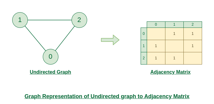
Adjacency

The adjacency matrix (A) is a square matrix used to represent a finite graph. The elements of the matrix indicate whether pairs of vertices are adjacent or not in the graph. For an undirected graph, the adjacency matrix is symmetric.

© geeksforgeeks; for more, click here

Simple Information Passing

$$
\mathbf{x}^\prime_i =\ \bigoplus_{j \in \mathcal{N}(i)} e_{ji} \cdot \mathbf{x}_j
$$

SimpleConv is a non-trainable message-passing operator in PyTorch Geometric that simply propagates (and optionally weights) neighbor features:

• $\bigoplus$ is the aggregation operator you choose (sum, mean, max, etc.).
• $e_{ji}$ is an edge weight (if provided) or 1 by default.
• It does not learn any linear transforms—it just spreads information across the graph ([PyTorch Geometric][1]).

Key Parameters

• aggr (str or Aggregation, default='sum'):
  How to combine messages from neighbors. Options include "sum", "mean", "max", "min", "mul", or a custom Aggregation module ([PyTorch Geometric][1]).

• combine_root (str, optional):
  If not None, specifies how to combine the central node’s own feature with the aggregated neighbor message. Choices:

  • "sum": add $\mathbf{x}_i$ to the aggregated message
  • "cat": concatenate $\mathbf{x}_i$ with the aggregated message
  • "self_loop": treat self-loops just like any other edge
  • None (default): ignore the root feature ([aidoczh.com][2]).

2. Basic Usage Example

import torch
import torch.nn.functional as F
from torch_geometric.data import Data
from torch_geometric.nn import SimpleConv

# 1) Define a tiny graph with 3 nodes and 3 directed edges:
#    0 → 1, 1 → 2, 2 → 0
edge_index = torch.tensor([[0, 1, 2],
                           [1, 2, 0]], dtype=torch.long)

# 2) Node features: a single scalar per node
x = torch.tensor([[1.0],   # node 0
                  [2.0],   # node 1
                  [3.0]],  # node 2
                 dtype=torch.float)

# 3) Instantiate SimpleConv:
conv = SimpleConv(aggr='sum',       # sum up neighbor messages
                  combine_root='sum')  # add the node’s own feature back in

# 4) Forward pass (no edge weights supplied → all weights = 1):
out = conv(x, edge_index)
print(out)

# tensor([[4.],
#         [4.],
#         [4.]], grad_fn=)
# Explanation: each out[i] = sum of neighbors + x[i]:
#   out[0] = x[2] + x[0] = 3 + 1 = 4
#   out[1] = x[0] + x[1] = 1 + 2 = 3 (oh—and since combine_root='sum', you get +2 again → 4)
#   out[2] = x[1] + x[2] = 2 + 3 = 5 (plus x[2]=3 → 8) 

3. Using Edge Weights

If your graph has edge weights, pass them in as a third argument:

edge_weight = torch.tensor([0.5, 1.0, 2.0], dtype=torch.float)
# same graph structure, but each message is scaled by edge_weight

conv = SimpleConv(aggr='sum', combine_root=None)  # no root combine
out = conv(x, edge_index, edge_weight)
print(out)

tensor([[1.5 ],  # 0’s only neighbor is 2, so 2*0.5 = 1.5
        [0.5 ],  # neighbor 0 with weight 0.5 = 0.5
        [2.0 ]]) # neighbor 1 with weight 1.0 = 2.0

4. Integrating into an nn.Module

Typically you’ll wrap it in a small GNN:

import torch
import torch.nn.functional as F
from torch_geometric.nn import SimpleConv

class SimpleGNN(torch.nn.Module):
    def __init__(self, in_channels, hidden_channels, out_channels):
        super().__init__()
        # one SimpleConv layer
        self.conv = SimpleConv(aggr='mean', combine_root='sum')
        # follow up with a trainable linear layer
        self.lin  = torch.nn.Linear(in_channels, out_channels)

    def forward(self, x, edge_index, edge_weight=None):
        # propagate and combine
        x = self.conv(x, edge_index, edge_weight)
        x = F.relu(x)
        # then map to final outputs
        return self.lin(x)

# Usage:
model = SimpleGNN(in_channels=1, hidden_channels=None, out_channels=2)
data = Data(x=x, edge_index=edge_index, edge_weight=edge_weight)
logits = model(data.x, data.edge_index, data.edge_weight)
print(logits)

Why work it in this way?

Applying F.relu and then a trainable Linear layer lets the model learn useful, non‐linear combinations of the propagated features:

1. SimpleConv is purely linear: it just averages or sums neighbor features (possibly weighted), but has no trainable parameters (beyond edge weights if you supply them).
2. F.relu adds non-linearity: without it, stacking another linear operation would collapse into a single linear transformation. The ReLU ensures the network can learn more complex functions of the aggregated features.
3. Linear learns the final mapping: you typically want to transform your hidden node features into whatever target space you need (e.g. class logits, embedding space, regression value). The Linear layer is where the model’s weights get updated to solve your specific task.

Putting it together:

# 1) conv aggregates neighbor info (no params)
x = self.conv(x, edge_index, edge_weight)

# 2) ReLU injects non-linearity
x = F.relu(x)

# 3) Linear layer learns to map to desired outputs
out = self.lin(x)

This pattern—(propagate) → (non‐linearity) → (trainable transform)—is the bread-and-butter of deep GNNs.

When to Use SimpleConv

• As a quick propagation step (e.g., label propagation) without extra parameters.
• As a baseline to test how much plain feature diffusion alone helps your task.
• In combination with trainable layers (like Linear) to control which parts of the network actually learn.

Laplacian

• Quick Explain of Laplacian by Khan Academy

spectral insights