nCov(新冠状病毒数据获取与可视化)
nCov(新冠状病毒数据获取与可视化)
1 Loading Packages
|
2 Data acquiring
|
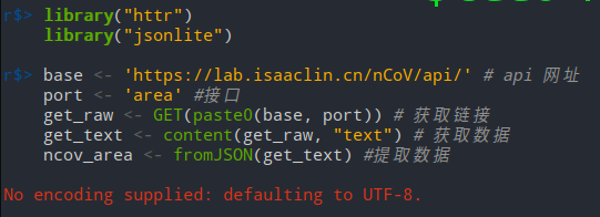
3 Data
|
這一步可能會因爲網絡問題而下載數據失敗. 可以直接用瀏覽器下載RDS, 然後本地讀取
下載地址: https://github.com/pzhaonet/ncov/raw/master/static/data-download/ncov.RDS
讀取方式:
|
讀取數據了, 就是喜聞樂見的, 清洗和可視化了
|
这里的时间困惑了我很久. 表格里的时间, 举例: 1583295001876, 通过as.Date.POSIXct 转化以后,成了"52142-08-15". 通过删除后面3位数, 876, 及可获得正确时间"2020-03-04". 我也不知道为什么
|
加上几个别的数据
|
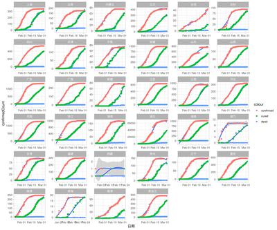
同样的方法看看别的省:
|
All Provinces
|
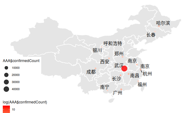
4 map
China city
cn_city_map.rds is required:
Specific Date is comming from GuangchuangYu
location: https://github.com/GuangchuangYu/map_data
But as you know, downloading Data from Github is preaty slow.
|
Take 湖北 as an example:
|
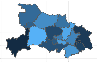
Adding nCov information
|
 |
 |
|---|
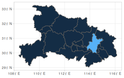
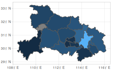
China Province
Data is shared by : skyme
Download locaktion: Click Here!
|
Location for main City (Data is from skyme)
|
|
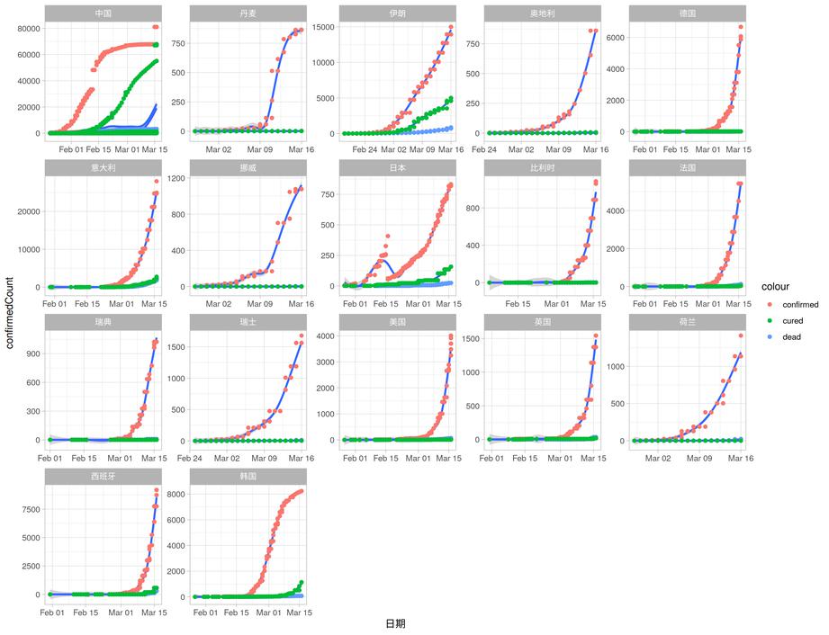
5 世界
|
Keep the countries which aboves 1000 confiremed cases.
|
nCov(新冠状病毒数据获取与可视化)


