PCA and PCoA

PCA

PCA

1 prcomp

## install ggbioplot
## remotes::install_github("vqv/ggbiplot")
## install.packages('plyr')

library(plyr)
library(ggbiplot)

data(wine)
wine.pca <- prcomp(wine, scale. = TRUE)
## bioplot
ggbiplot(wine.pca, obs.scale = 1, var.scale = 1,
         groups = wine.class, ellipse = TRUE, circle = TRUE) +
  scale_color_discrete(name = '') +
  theme_light()+ theme(axis.title = element_text(size=10))


# var.axis = F to remove the varible axis on the center.

1.1 Arguments

ggbiplot(pcobj, choices = 1:2, scale = 1, pc.biplot =
TRUE, obs.scale = 1 - scale, var.scale = scale, groups =
NULL, ellipse = FALSE, ellipse.prob = 0.68, labels =
NULL, labels.size = 3, alpha = 1, var.axes = TRUE, circle
= FALSE, circle.prob = 0.69, varname.size = 3,
varname.adjust = 1.5, varname.abbrev = FALSE, ...)
pcobj # prcomp()或princomp()返回结果
choices # 选择轴，默认1：2
scale # covariance biplot (scale = 1), form biplot (scale = 0). When scale = 1, the inner product between the variables approximates the covariance and the distance between the points approximates the Mahalanobis distance.
obs.scale # 标准化观测值
var.scale # 标准化变异
pc.biplot # 兼容 biplot.princomp()
groups # 组信息，并按组上色
ellipse # 添加组椭圆
ellipse.prob # 置信区间
labels #向量名称
labels.size #名称大小
alpha  #点透明度 (0 = TRUEransparent, 1 = opaque)
circle #绘制相关环(only applies when prcomp was called with scale = TRUE and when var.scale = 1)
var.axes  #绘制变量线-菌相关
varname.size  #变量名大小
varname.adjust #标签与箭头距离 >= 1 means farther from the arrow
varname.abbrev # 标签是否缩写

2 Psych

library(psych)
library(ggplot2)

# calculate PCA
PC <- principal(wine, nfactors=2, rotate ="none")
pc <- data.frame(PC$scores)

# calculate the location of labels
Label_pos <- aggregate(cbind(PC1, PC2) ~ wine.class, data=pc, FUN=median)

# Plot the PCA scatter graph
ggplot(pc, aes(x=PC1, y=PC2,color=wine.class )) + 
    geom_point(size=4,alpha=0.5)+ theme_light() +  
    geom_label(data = Label_pos, aes(label = wine.class), alpha = .3)+ 
    stat_ellipse(lwd=1,level = 0.95, alpha= .8, linetype = 4)

3 qplot

library(ggplot2)
qplot(x=PC1,y=PC2, data=pc,colour=factor(wine.class))+theme(legend.position="none")+stat_ellipse(lwd=1,level = 0.8)

More

library(ggbiplot)
library(ggthemes)
library(patchwork)

data(wine)
wine.pca <- prcomp(wine, scale. = TRUE)
## bioplot
TB= data.frame(wine.pca$x)
TB$class = wine.class

p0 <- ggbiplot(wine.pca, obs.scale = 1, var.scale = 1,
        groups = wine.class, ellipse = TRUE, circle = TRUE) +
        scale_color_discrete(name = '') +
        theme_light()+theme(legend.position = 'none',
        axis.title=element_blank())

p1 <- ggplot() +
        geom_density(data=TB, aes(x=PC1,fill=class),alpha=0.5) +
        theme_map() +
        theme(legend.position = 'none')

p2 <- ggplot() +
        geom_density(data=TB, aes(x=PC2,fill=class),alpha=0.5)  +
        theme_map() +theme(legend.position = 'none') +
        coord_flip()  +  scale_y_reverse()

p3 <- ggplot(TB, aes(x=class,y=PC1)) +
        geom_tufteboxplot(aes(color=class),median.type = "line",
          hoffset = 0, width = 3) +
        coord_flip()+ theme_map()+
        theme(legend.position = 'none')

p4 <- ggplot(TB, aes(x=class,y=PC2)) +
        geom_tufteboxplot(aes(color=class),median.type = "line",
          hoffset = 0, width = 3) +
        theme_map()+
        theme(legend.position = 'none')


TB= data.frame(wine.pca$x)
TB$class = wine.class

GGlay <-
"#BBBBBB#
CAAAAAAE
CAAAAAAE
CAAAAAAE
CAAAAAAE
CAAAAAAE
CAAAAAAE
##DDDDDD#"
p0+p1+p2+p3+p4  +plot_layout(design = GGlay)

PCoA

What's different between PCA and PCoA?

Principal Component Analysis (PCA) and Principal Coordinates Analysis (PCoA, also known as Multidimensional Scaling, MDS) are both techniques used for dimensionality reduction, which is the process of reducing the number of random variables under consideration by obtaining a set of principal variables. However, they are used in different contexts and have different underlying methodologies.

PCA is a technique that is used when you have a multivariate data set and you want to identify new variables that will represent the variability of your entire data set as much as possible. The new variables, or principal components, are linear combinations of the original variables. PCA operates on a covariance (or correlation) matrix, which implies that it is a parametric method.

On the other hand, PCoA is a method used in ecology and biology to transform a matrix of distances (or dissimilarities) between samples into a new set of orthogonal axes, the most important of which can be plotted against each other. PCoA can be applied to any symmetric distance or dissimilarity matrix. Unlike PCA, PCoA is non-parametric and makes no assumptions about the distribution of the original variables.

So, the main difference lies in the type of data they work with: PCA works with the actual data matrix and is used when you have a set of observations and measurements, while PCoA works with a matrix of pairwise distances and is used when you have a set of pairwise dissimilarities (like geographical distances between cities or genetic distances between individuals or species).

© ChatGPT4

Interesting

PCA in Python

Main PCA research and Plot

import pandas as pd
from sklearn.decomposition import PCA
from sklearn.preprocessing import StandardScaler
from sklearn.datasets import load_wine
import matplotlib.pyplot as plt

# Step 1: Load the wine dataset
wine_data = load_wine()
df = pd.DataFrame(data=wine_data.data, columns=wine_data.feature_names)

# Step 2: Standardize the data (optional but recommended)
scaler = StandardScaler()
scaled_data = scaler.fit_transform(df)

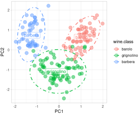
# Run the PCA with 3 components
pca = PCA(n_components=2)  # Reduce to 2 dimensions for visualization
principal_components = pca.fit_transform(scaled_data)
pca_df = pd.DataFrame(data=principal_components, columns=['PC1', 'PC2'])
pca_df['target'] = wine_data.target
# Create a scatter plot with color based on the target class
scatter = plt.scatter(pca_df['PC1'], pca_df['PC2'], c=pca_df['target'], cmap='viridis', edgecolor='k', alpha=0.7)

# Adding labels and title
plt.xlabel('Principal Component 1')
plt.ylabel('Principal Component 2')
plt.title('PCA of Wine Dataset')

# Add a color bar to indicate the different classes
plt.colorbar(scatter, ticks=[0, 1, 2], label='Wine Class')

# Optionally, add a legend (if your target classes are categorical)
# legend = plt.legend(*scatter.legend_elements(), title="Classes")
# plt.gca().add_artist(legend)

# Show the plot
plt.grid(True)
plt.show()

By checking the raw data, each column is feature, row is element.

Index	Alcohol	Malic Acid	…	OD280/OD315 of Diluted Wines	Proline
0	14.23	1.71	…	3.92	1065.0
1	13.20	1.78	…	3.40	1050.0
2	13.16	2.36	…	3.17	1185.0
3	14.37	1.95	…	3.45	1480.0
4	13.24	2.59	…	2.93	735.0
…	…	…	…	…	…
173	13.71	5.65	…	1.74	740.0
174	13.40	3.91	…	1.56	750.0
175	13.27	4.28	…	1.56	835.0
176	13.17	2.59	…	1.62	840.0
177	14.13	4.10	…	1.60	560.0

Explained Variance Ratio

# Step 3: Perform PCA
pca = PCA()  # By default, PCA will consider all components
pca.fit(scaled_data)

# Step 4: Get the explained variance ratio for each component
explained_variance_ratio = pca.explained_variance_ratio_

# Step 5: Create a DataFrame to store component contributions
component_contributions = pd.DataFrame({
    'Principal Component': [f'PC{i+1}' for i in range(len(explained_variance_ratio))],
    'Explained Variance Ratio': explained_variance_ratio
})

# Step 6: Sort the components by their contribution (explained variance ratio)
component_contributions_sorted = component_contributions.sort_values(by='Explained Variance Ratio', ascending=False)

# Display the sorted components
print(component_contributions_sorted)

# Step 7: Optionally, you can plot the explained variance ratio to visualize
plt.figure(figsize=(8, 6))
plt.bar(range(1, len(explained_variance_ratio) + 1), explained_variance_ratio, alpha=0.7, align='center',
        label='individual explained variance')
plt.step(range(1, len(explained_variance_ratio) + 1), explained_variance_ratio.cumsum(), where='mid',
         label='cumulative explained variance')
plt.ylabel('Explained variance ratio')
plt.xlabel('Principal components')
plt.legend(loc='best')
plt.tight_layout()
plt.show()

Index	Principal Component	Explained Variance Ratio
0	PC1	0.361988
1	PC2	0.192075
2	PC3	0.111236
3	PC4	0.070690
4	PC5	0.065633
5	PC6	0.049358
6	PC7	0.042387
7	PC8	0.026807
8	PC9	0.022222
9	PC10	0.019300
10	PC11	0.017368
11	PC12	0.012982
12	PC13	0.007952

Contribution of Each Features

import numpy as np

# adding a new column for test.
df2 = df.copy()
df2['test'] = 0
# Perform PCA
pca = PCA()
pca.fit(df2)
# Get the loadings (components)
loadings = pca.components_.T
# Calculate the contribution of each feature
feature_contributions = np.sum(np.abs(loadings), axis=1)
# Create a DataFrame to rank features
feature_importance_df = pd.DataFrame({
    'Feature': wine_data.feature_names + ['test'],
    'Contribution': feature_contributions
})
feature_importance_df = feature_importance_df.sort_values(by='Contribution', ascending=False).reset_index(drop=True)
# Rank features by their contribution

We can find the this contribution results, the text column doesn’t has any of contribution in variation since all values are equals to 1.

	Feature	Contribution
0	flavanoids	2.640230
1	od280/od315_of_diluted_wines	2.066036
2	total_phenols	2.050567
3	malic_acid	1.991115
4	proanthocyanins	1.981272
5	color_intensity	1.867953
6	alcohol	1.849138
7	hue	1.807356
8	magnesium	1.707784
9	ash	1.558561
10	alcalinity_of_ash	1.551888
11	nonflavanoid_phenols	1.430382
12	malic_acid	1.204709
13	test	1.000000