Linear Regression

Regression in R

Reference: Multiple linear regression made simple; 2021

linear equation with one unknown

test data: mpg form ggplot2

Quick start

library(ggplot2)
## calculating the model
model_mpg <- lm(formula = hwy ~ displ, data = mpg)

print(model_mpg)

Call:
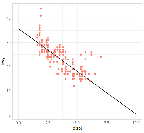
lm(formula = hwy ~ displ, data = mpg)

Coefficients:
(Intercept)        displ  
     35.698       -3.531

As we can see above, the function is

$$
y = -3.531x+35.698
$$

summary(model_mpg)

Call:
lm(formula = hwy ~ displ, data = mpg)

Residuals:
    Min      1Q  Median      3Q     Max
-7.1039 -2.1646 -0.2242  2.0589 15.0105

Coefficients:
            Estimate Std. Error t value Pr(>|t|)    
(Intercept)  35.6977     0.7204   49.55   <2e-16 ***
displ        -3.5306     0.1945  -18.15   <2e-16 ***
---
Signif. codes:  0 ‘**\*’ 0.001 ‘**’ 0.01 ‘*’ 0.05 ‘.’ 0.1 ‘ ’ 1

Residual standard error: 3.836 on 232 degrees of freedom
Multiple R-squared:  0.5868,	Adjusted R-squared:  0.585
F-statistic: 329.5 on 1 and 232 DF,  p-value: < 2.2e-16

Plot

Formula <- function(x){
  -3.531*x+35.698
}

x=c(0:10)

## Origiaml point
ggplot() + geom_point(data=mpg, aes(x=displ, y=hwy),color='salmon') +
  theme_light()+  
  # regression model
  geom_line(aes(x=x,y=Formula(x)))

Practice

P value and R²

n<-c(0.0000, 0.0310, 0.0130, 0.0450, 0.0570, 0.0540, 0.1100, 0.0930, 0.1100, 0.1030, 0.1350, 0.1650)
m = c(1:length(n))
df<-as.data.frame(cbind(m,n))

model_mpg <- lm(formula = n ~ m, data = df)

print(model_mpg)
summary(model_mpg)

Call:
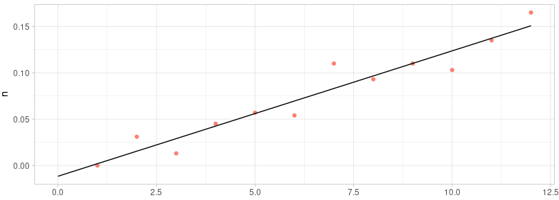
lm(formula = n ~ m, data = df)

Coefficients:
(Intercept)            m  
   -0.01162      0.01353  



Call:
lm(formula = n ~ m, data = df)

Residuals:
      Min        1Q    Median        3Q       Max
-0.020694 -0.006615 -0.001036  0.005432  0.026901

Coefficients:
             Estimate Std. Error t value Pr(>|t|)    
(Intercept) -0.011621   0.008968  -1.296    0.224    
m            0.013531   0.001219  11.105 6.04e-07 ***
---
Signif. codes:  0 ‘\***’ 0.001 ‘**’ 0.01 ‘*’ 0.05 ‘.’ 0.1 ‘ ’ 1

Residual standard error: 0.01457 on 10 degrees of freedom
Multiple R-squared:  0.925,	Adjusted R-squared:  0.9175
F-statistic: 123.3 on 1 and 10 DF,  p-value: 6.036e-07

We can know that the function of this result is:$y=0.01353x-0.01162$
The R² = 0.925, p-value = 6.036e-07
According to the P-value, we could say that the x and y are significantly correlated. Based on the R², we can say the fitting result is pretty reliable.

To be notice that for the slope, the sd is 0.00012 and for the intercept, the sd is 0.0090. They are independent.

Turn R to P

There are two online tools which can calculate the P value from R (not R²):

• Tool 1
• Tool 2

And there are also code for calculate the p value from R²:
Reference: Jake Westfall; 2014

The formula is:
$$
r^ 2 ≈ Beta(\frac{V_ n}{2}, \frac{V_ d}{2})
$$

V_n and V_d are the numerator and denominator degrees of freedom, respectively, for the associated F-statistic.

# Rsqr is R squared value
# df is Number of elements minus 2
1 - pbeta(Rsqr, 1/2, df/2)

Runs test

library(ggplot2)
library(DescTools)

Formula <- function(x){
  0.01353*x-0.01162
}

x=c(0:12)

## Origiaml point
ggplot() + geom_point(data=df, aes(x=m, y=n),color='salmon') +
  theme_light()+  
  # regression model
  geom_line(aes(x=x,y=Formula(x)))

TMP = n - Formula(df$m)
TMP[which(TMP>0)] = 1
TMP[which(TMP<0)] = -1
RunsTest(TMP, alternative = "less")

Runs Test for Randomness

data:  TMP
runs = 8, m = 7, n = 5, p-value = 0.8535
alternative hypothesis: true number of runs is less than expected

This runs test for randomness is achieved by divided the raw data into two groups, the elements larger than the predicted values are assigned into 1, smaller elements are assigned into -1. After that, we only use the “less” part the calculate the p value and find which is not significant. So, we can say that they are not significant different and the regression function is acceptable.

PS: this is are exactly Prism suppose to run the runs test

Confidence and prediction intervals are often formed to answer questions such as the above. Intervals allow one to estimate a range of values that can be said with reasonable confidence (typically 95%) contains the true population parameter. It should be noted that although the questions above sound similar, there is a difference in estimating a mean response and predicting a new value. This difference will be seen in the interval equations. This post will explore confidence and prediction intervals as well as the confidence ‘bands’ around a linear regression line.
rpubs.com: Confidence Interval of the linear regression

library(car)

reg.conf.intervals <- function(x, y, cof=0.95) {
  n <- length(y) # Find length of y to use as sample size
  lm.model <- lm(y ~ x) # Fit linear model

  # Extract fitted coefficients from model object
  b0 <- lm.model$coefficients[1]
  b1 <- lm.model$coefficients[2]

  # Find SSE and MSE
  sse <- sum((y - lm.model$fitted.values)^2)
  mse <- sse / (n - 2)

  t.val <- qt(cof, n - 2) # Calculate critical t-value

  # Fit linear model with extracted coefficients
  x_new <- 1:max(x)
  y.fit <- b1 * x_new + b0

  # Find the standard error of the regression line
  se <- sqrt(sum((y - y.fit)^2) / (n - 2)) * sqrt(1 / n + (x - mean(x))^2 / sum((x - mean(x))^2))

  # Fit a new linear model that extends past the given data points (for plotting)
  x_new2 <- 1:max(x + 100)
  y.fit2 <- b1 * x_new2 + b0

  # Warnings of mismatched lengths are suppressed
  slope.upper <- suppressWarnings(y.fit2 + t.val * se)
  slope.lower <- suppressWarnings(y.fit2 - t.val * se)

  # Collect the computed confidence bands into a data.frame and name the colums
  bands <- data.frame(cbind(slope.lower, slope.upper))
  colnames(bands) <- c('Lower Confidence Band', 'Upper Confidence Band')

  # Plot the fitted linear regression line and the computed confidence bands
  plot(x, y, cex = 1.75, pch = 21, bg = 'gray')
  lines(y.fit2, col = 'black', lwd = 2)
  lines(bands[1], col = 'blue', lty = 2, lwd = 2)
  lines(bands[2], col = 'blue', lty = 2, lwd = 2)

  return(bands)
}

conf.intervals <- reg.conf.intervals(df$m, df$n)

Zach, 2020

Outliers

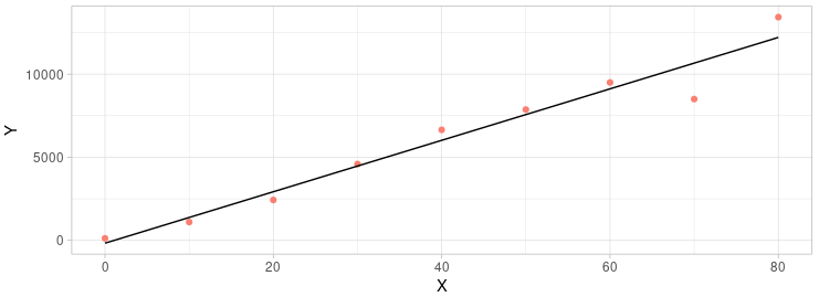
To check the outliers we could use the chauvenet’s test which is based on the t-test. The basic idea is to check the t-distribution of the difference between the real number and the expected number. The number is different from the expected and can’t pass the chauvenet’s test been seam as outliers.

As you can see from the graph above (the code for the plot is attached below), the last two points are far from the regression line. Mandatory discarding both of them would be arbitrary and inconvincible. But it would be a good idea to use the chauvenet’s test to decide which one should be kept and which one should be discarded.

# define the chauvenet's test function

chauvenet_test <- function(A){
	Dmax = abs(qnorm(1/4/length(A)))
	Outer = A[abs(scale(A))>= abs(Dmax)]
	Z_out = abs(scale(A))[abs(scale(A))>= abs(Dmax)]
	P_val = 1- pnorm(abs(scale(A)), lower.tail = T)
	print(paste("Dmax:", Dmax))
	print(paste("Outliners:",Outer))
	print(paste("Zscore:", Z_out))
	print(paste("P value:", P_val))
	return(Outer)
}

## Create the date

Y = c(120, 1100, 2430, 4590, 6650, 7870, 9500, 8500, 13430)
X = c(0, 10, 20, 30, 40, 50, 60, 70, 80)
TB = data.frame(X=X, Y=Y)
l_model <- lm(Y~X, data=TB)
summary(l_model)

Formula <- function(x){
   154.77 *x-169.56
}


## Origiaml point
ggplot() + geom_point(data=TB, aes(x=X, y=Y),color='salmon') +
  theme_light()+  
  # regression model
  geom_line(aes(x=X,y=Formula(X)))

Call:
lm(formula = Y ~ X, data = TB)

Residuals:
    Min      1Q  Median      3Q     Max
-2164.1  -278.1   289.6   383.6  1218.2

Coefficients:
            Estimate Std. Error t value Pr(>|t|)    
(Intercept)  -169.56     624.28  -0.272    0.794    
X             154.77      13.11  11.803  7.1e-06 ***
---
Signif. codes:  0 ‘\***’ 0.001 ‘**’ 0.01 ‘*’ 0.05 ‘.’ 0.1 ‘ ’ 1

Residual standard error: 1016 on 7 degrees of freedom
Multiple R-squared:  0.9522,	Adjusted R-squared:  0.9453
F-statistic: 139.3 on 1 and 7 DF,  p-value: 7.105e-06

Though the P-value and R² tell us that the fitness result is very promising, we still want to see how the outlier affects the fitness.

chauvenet_test(Y - Formula(X))

The output of the chauvenet_test

[1] "Dmax: 1.91450582505556"
[1] "Outliners: -2164.34"
[1] "Zscore: 2.27790206887637"
[1] "P value: 0.380218526950083"  "P value: 0.384907967278372"
[3] "P value: 0.300921524723487"  "P value: 0.451166958976122"
[5] "P value: 0.254009368820307"  "P value: 0.37561761649201"  
[7] "P value: 0.343240779142229"  "P value: 0.0113662064986361"
[9] "P value: 0.0999076632824158"
[1] -2164.34

which(c(Y - Formula(X))==chauvenet_test(Y - Formula(X)))

[1] 8

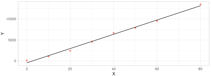
We can see the the 8^th element in Y could be discarded. Let’s we run everything again without it.

l_model <- lm(Y~X, data=TB[-8,])
summary(l_model)

Formula <- function(x){
   169.411 *x-429.900
}

## Origiaml point
ggplot() + geom_point(data=TB[-8,], aes(x=X, y=Y),color='salmon') +
  theme_light()+  
  # regression model
  geom_line(aes(x=X,y=Formula(X)))

Call:
lm(formula = Y ~ X, data = TB[-8, ])

Residuals:
   Min     1Q Median     3Q    Max
-528.3 -186.7 -113.3  304.4  549.9

Coefficients:
            Estimate Std. Error t value Pr(>|t|)    
(Intercept) -429.900    239.097  -1.798    0.122    
X            169.411      5.432  31.188 7.22e-08 ***
---
Signif. codes:  0 ‘\***’ 0.001 ‘**’ 0.01 ‘*’ 0.05 ‘.’ 0.1 ‘ ’ 1

Residual standard error: 383.6 on 6 degrees of freedom
Multiple R-squared:  0.9939,	Adjusted R-squared:  0.9928
F-statistic: 972.7 on 1 and 6 DF,  p-value: 7.217e-08

We can see that the fitness was much better than before when we discard the 8^th element. The R² is larger than before and P-value is smaller than before. Seams we had a better result than before.

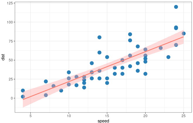
Confidential intervals

There is two way you can do for draw confidential intervals. One is using ggplot2. The functions geom_smooth could help you finish it very elegantly. Another way is to follow the steps from rpubs which calculate it by yourself.

In ggplot

Let’s see how can we achieve it with ggplot2. The threshold of the interval is 0.95 which could be changed in level =

library(ggplot2)
data("cars")
ggplot(cars, aes(x=speed, y=dist)) +
  geom_point(color='#2980B9', size = 4) +
  geom_smooth(method=lm, color='salmon', fill= "#ffa4a3",  level = 0.95)+
  theme_bw()

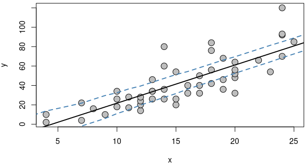
Calculating confidence interval by yourself:

Points from upper and lower side would be calculated and stored.

reg.conf.intervals <- function(x, y, CI=0.975) {
  n <- length(y) # Find length of y to use as sample size
  lm.model <- lm(y ~ x) # Fit linear model

  # Extract fitted coefficients from model object
  b0 <- lm.model$coefficients[1]
  b1 <- lm.model$coefficients[2]

  # Find SSE and MSE
  sse <- sum((y - lm.model$fitted.values)^2)
  mse <- sse / (n - 2)

  t.val <- qt(CI, n - 2) # Calculate critical t-value

  # Fit linear model with extracted coefficients
  x_new <- 1:max(x)
  y.fit <- b1 * x_new + b0

  # Find the standard error of the regression line
  se <- sqrt(sum((y - y.fit)^2) / (n - 2)) * sqrt(1 / n + (x - mean(x))^2 / sum((x - mean(x))^2))

  # Fit a new linear model that extends past the given data points (for plotting)
  x_new2 <- 1:max(x + 100)
  y.fit2 <- b1 * x_new2 + b0

  # Warnings of mismatched lengths are suppressed
  slope.upper <- suppressWarnings(y.fit2 + t.val * se)
  slope.lower <- suppressWarnings(y.fit2 - t.val * se)

  # Collect the computed confidence bands into a data.frame and name the colums
  bands <- data.frame(cbind(slope.lower, slope.upper))
  colnames(bands) <- c('Lower Confidence Band', 'Upper Confidence Band')

  # Plot the fitted linear regression line and the computed confidence bands
  plot(x, y, cex = 1.75, pch = 21, bg = 'gray')
  lines(y.fit2, col = 'black', lwd = 2)
  lines(bands[1], col = 'steelblue', lty = 2, lwd = 2)
  lines(bands[2], col = 'steelblue', lty = 2, lwd = 2)

  return(bands)
}

conf.intervals <- reg.conf.intervals(cars$speed, cars$dist)
head(conf.intervals)

Lower Confidence Band Upper Confidence Band
1            -33.350170              6.056798
2            -29.417761              9.989207
3            -21.327925              9.764188
4            -17.395516             13.696597
5            -12.154300             16.320197
6             -6.971285             19.002000

Quadratic Equation

Standard Equation:
$$
y=ax^2+bx+c
$$

model_mpg1 <- lm(formula = hwy ~ I(displ^2), data = mpg)
model_mpg2 <- lm(formula = hwy ~ I(displ^2) + displ, data = mpg)

model_mpg1:

Call:
lm(formula = hwy ~ I(displ^2), data = mpg)

Coefficients:
(Intercept)   I(displ^2)  
     29.324       -0.429  

model_mpg2:

Call:
lm(formula = hwy ~ I(displ^2) + displ, data = mpg)

Coefficients:
(Intercept)   I(displ^2)        displ  
     49.245        1.095      -11.760  

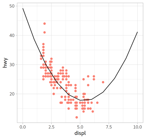
plot

Formula1 <- function(x){
  model_mpg1$coefficients[2]*x^2 + model_mpg1$coefficients[1]
}

Formula2 <- function(x){
  model_mpg2$coefficients[2]*x^2 + model_mpg2$coefficients[3]*x +model_mpg2$coefficients[1]
}

ggplot() + geom_point(data=mpg, aes(x=displ, y=hwy),color='salmon') +
  theme_light()+  
  # regression model
  geom_line(aes(x=x,y=Formula1(x)))

ggsave('')
ggplot() + geom_point(data=mpg, aes(x=displ, y=hwy),color='salmon') +
  theme_light()+  
  # regression model
  geom_line(aes(x=x,y=Formula2(x)))

	model_mpg1	model_mpg2
Formula	$y=-0.429x^{2}+29.324$	$y=1.095x^{2} -11.760x + 49.245$
Plot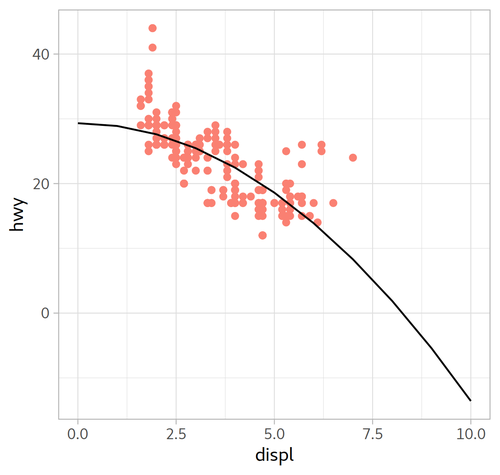

cor

cor()

R²

谦瑞数据 2019

mylr = function(x,y){
  x_mean = mean(x)
  y_mean = mean(y)
  xy_mean = mean(x*y)
  xx_mean = mean(x*x)
  yy_mean = mean(y*y)

  m = (x_mean*y_mean - xy_mean)/(x_mean^2 - xx_mean)
  b = y_mean - m*x_mean

  f = m*x+b# 线性回归方程
  sst = sum((y-y_mean)^2)
  sse = sum((y-f)^2)
  ssr = sum((f-y_mean)^2)
  result = c(m,b,sst,sse,ssr)
  names(result) = c('m','b','sst','sse','ssr')
  result['ssr']/result['sst']
}



x = c(60,34,12,34,71,28,96,34,42,37)

y = c(301,169,47,178,365,126,491,157,202,184)

一元多次回归方程自动扫描

T test and P value: 数据挖掘运爷

Functions:

Click to see

mylr = function(x,y){
  x_mean = mean(x)
  y_mean = mean(y)
  xy_mean = mean(x*y)
  xx_mean = mean(x*x)
  yy_mean = mean(y*y)

  m = (x_mean*y_mean - xy_mean)/(x_mean^2 - xx_mean)
  b = y_mean - m*x_mean

  f = m*x+b# 线性回归方程
  sst = sum((y-y_mean)^2)
  sse = sum((y-f)^2)
  ssr = sum((f-y_mean)^2)
  result = c(m,b,sst,sse,ssr)
  names(result) = c('m','b','sst','sse','ssr')
  result['ssr']/result['sst']
}

F_equation <- function(X,Formula){
  eval(parse(text = Formula))
}

LMEE <- function(TB,Times){
  colnames(TB)=c("X","Y")

  Group_X = "X"
  for(i in c(2:Times)){
    X_i = paste("I(X^",i,")",sep="")
    Group_X = paste(Group_X,X_i,sep=" + ")
  }
  str_lm = paste("lm(Y ~",Group_X, ', data=TB)', sep=' ')
  model = eval(parse(text = str_lm))

  Formula = model$coefficients[1]
  for(i in c(Times:1)){
    X_tmp = paste(model$coefficients[i+1], " * X^", i, sep="")
    Formula = paste(Formula,X_tmp,sep="+")
  }
  # T value
  tstats <- coef(model) / sqrt(diag(vcov(model)))
  Tvalue = matrix(tstats)[2]
  # P value
  pvalue <- 2 * pt(abs(tstats), df = df.residual(fit), lower.tail = FALSE)
  Pvalue <- matrix(pvalue)[2]

  R2 = mylr(TB$Y,F_equation(TB$X,Formula))

  result = c()
  result$R2      = R2[[1]]
  result$model   = model
  result$Tvalue  = Tvalue
  result$Pvalue  = Pvalue
  result$Formula =Formula

  return(result)
}


MEES <- function(TB, Times){
  colnames(TB)=c("X","Y")
  Result_TB = data.frame()
  for(i in c(1:Times)){
      Result_LMEE = LMEE(TB,i)
      Result_tmp = data.frame(Exp= i, P_value = Result_LMEE$Pvalue, R2= Result_LMEE$R2, F = Result_LMEE$Formula)
      Result_TB = rbind(Result_TB, Result_tmp)
  }

  return(Result_TB)
}

MEES_plot <- function(TB,TB_input, BY = 1, header="test"){
  colnames(TB)=c("X","Y")
  TB_Nna = na.omit(TB_input)
  XX = seq(from=min(TB$X), to =max(TB$X), by = BY)
  for(i in c(1:nrow(TB_Nna))){
    ggplot()+geom_point(data=TB,aes(x=X,y=Y))+
             geom_line(aes(x=XX, y=F_equation(XX, as.character(TB_Nna$F[i]))))
    ggsave(paste(header,i,".png",sep=""))
  }
}

Usage:

##Test Data
TB <- head(ChickWeight)[c(2,1)]

MEES(TB,4)
MEES_plot(TB,MEES(TB,4))

	Exp	P_value	R2	F
ssr	1	5.100486e-02	0.9641461	$40.2380952380953 + 4.78571428571428 * X$
1	2	5.100486e-02	0.9865977	43.5714285714286+0.250000000000001 * X^2+2.28571428571428 * X^1
11	3	1.550240e-08	0.9986254	41.904761904762+0.069444444444444 * X^3±0.791666666666658 * X^2+6.0912698412698 * X^1
12	4	3.012296e-02	0.9986254	41.904761904762+2.01944464079605e-16 * X^4+0.0694444444444399 * X^3±0.791666666666634 * X^2+6.09126984126975 * X^1
13	5	NaN	1.0000000	41.9999999999999±0.00625000000000004 * X^5+0.156250000000001 * X^4±1.29166666666667 * X^3+3.99999999999998 * X^2+0.516666666666805 * X^1

Logarithmic Regression

Modle <- lm(formula = hwy ~ log(displ,2) , data = mpg)

Call:
lm(formula = hwy ~ log(displ, exp(1)), data = mpg)

Coefficients:
       (Intercept)  log(displ, exp(1))  
             38.21              -12.57  

Modle <- lm(formula = Y ~ log(X+1), data = TB)

Formula <- function(x){
  Modle$coefficients[[2]]  * log(x-1) + Modle$coefficients[[1]]
}

X= seq(0,5000, by=2)

ggplot() + geom_point(data= TB, aes(x=X, y=Y)) +
  geom_point(aes(x=X, y= Formula(c(1:length(X)))), color="salmon")

drc

X <- TB$X
Y <- TB$Y

library(drc)

mod1<-drm(Y ~ X, fct=LL.2())
summary(mod1)

plot(X,Y)
lines(seq(0,5000, by=2), predict(mod1, data.frame(X=seq(0,5000, by=2))))

Test:

Google
s