Single cell RNA-Seq Practice: Seurat© Karobben

Single cell RNA-Seq Practice: Seurat

Single cell RNA-seq Data processing

This is my first time to learn siRNA-Seq. The protocol are based on Seurat. Please go and reading more information from Seurat. The codes are derectly copied from Seurat and so, if you are confuzed about my moves, please go to the link below and check by yourselves.

For new users of Seurat, we suggest starting with a guided walk through of a dataset of 2,700 Peripheral Blood Mononuclear Cells (PBMCs) made publicly available by 10X Genomics. This tutorial implements the major components of a standard unsupervised clustering workflow including QC and data filtration, calculation of high-variance genes, dimensional reduction, graph-based clustering, and the identification of cluster markers.
Seurat

Source code: © Seurat 2021

Downlaod Practice Data

Data set: Peripheral Blood Mononuclear Cells (PBMC) freely available from 10X Genomics.

wget https://cf.10xgenomics.com/samples/cell/pbmc3k/pbmc3k_filtered_gene_bc_matrices.tar.gz
tar -zxvf pbmc3k_filtered_gene_bc_matrices.tar.gz

tree filtered_gene_bc_matrices/hg19
filtered_gene_bc_matrices/hg19
├── barcodes.tsv
├── genes.tsv
└── matrix.mtx
head -n 4 filtered_gene_bc_matrices/hg19/*
==> filtered_gene_bc_matrices/hg19/barcodes.tsv <==
AAACATACAACCAC-1
AAACATTGAGCTAC-1
AAACATTGATCAGC-1
AAACCGTGCTTCCG-1

==> filtered_gene_bc_matrices/hg19/genes.tsv <==
ENSG00000243485	MIR1302-10
ENSG00000237613	FAM138A
ENSG00000186092	OR4F5
ENSG00000238009	RP11-34P13.7

==> filtered_gene_bc_matrices/hg19/matrix.mtx <==
%%MatrixMarket matrix coordinate real general
%
32738 2700 2286884
32709 1 4

Data loading

library(dplyr)
library(Seurat)
library(patchwork)

# Load the PBMC dataset
pbmc.data <- Read10X(data.dir = "filtered_gene_bc_matrices/hg19/")
# Initialize the Seurat object with the raw (non-normalized data).
pbmc <- CreateSeuratObject(counts = pbmc.data, project = "pbmc3k", min.cells = 3, min.features = 200)
pbmc
An object of class Seurat
13714 features across 2700 samples within 1 assay
Active assay: RNA (13714 features, 0 variable features)
What does data in a count matrix look like?
# Lets examine a few genes in the first thirty cells
pbmc.data[c("CD3D", "TCL1A", "MS4A1"), 1:30]
  3 x 30 sparse Matrix of class "dgCMatrix"

  CD3D  4 . 10 . . 1 2 3 1 . . 2 7 1 . . 1 3 . 2  3 . . . . . 3 4 1 5
  TCL1A . .  . . . . . . 1 . . . . . . . . . . .  . 1 . . . . . . . .
  MS4A1 . 6  . . . . . . 1 1 1 . . . . . . . . . 36 1 2 . . 2 . . . .
  
dense.size <- object.size(as.matrix(pbmc.data))
dense.size
sparse.size <- object.size(pbmc.data)
sparse.size
dense.size/sparse.size
  709591472 bytes
  29905192 bytes
  23.7 bytes
  

Standard pre-processing workflow

QC and selecting cells for further analysis

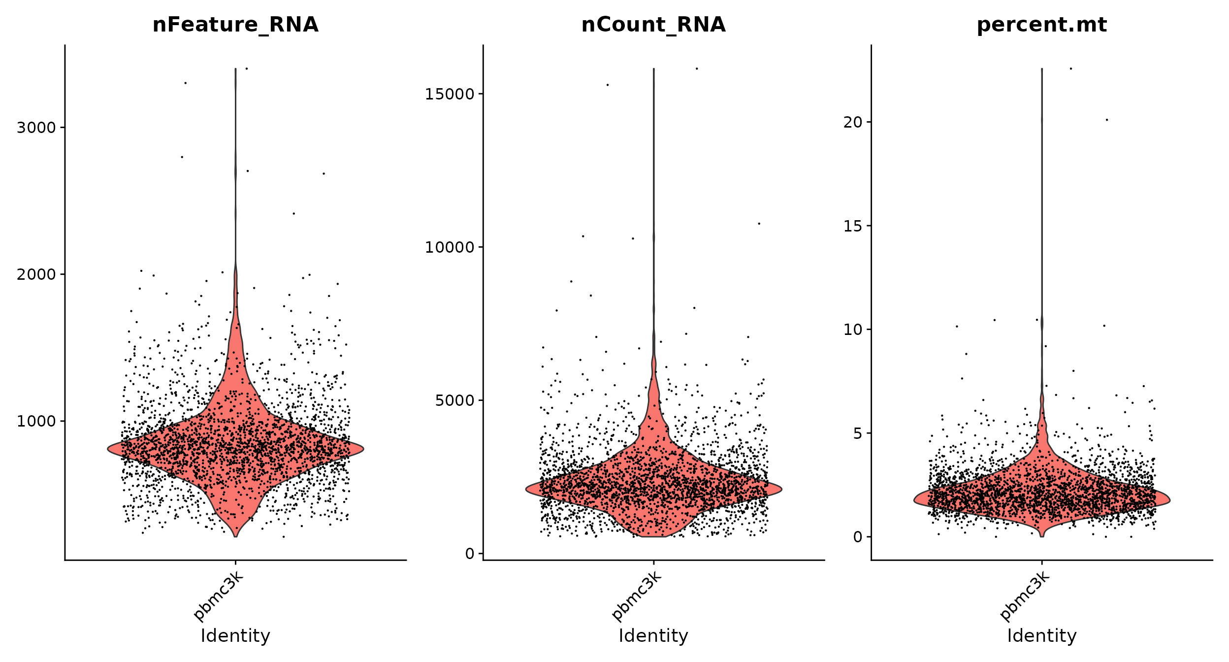
# The [[ operator can add columns to object metadata. This is a great place to stash QC stats
pbmc[["percent.mt"]] <- PercentageFeatureSet(pbmc, pattern = "^MT-")
VlnPlot(pbmc, features = c("nFeature_RNA", "nCount_RNA", "percent.mt"), ncol = 3)
Where are QC metrics stored in Seurat?
head(pbmc@meta.data, 5)
  
orig.identnCount_RNAnFeature_RNApercent.mt
<fct><dbl><int><dbl>
AAACATACAACCAC-1pbmc3k2419 7793.0177759
AAACATTGAGCTAC-1pbmc3k490313523.7935958
AAACATTGATCAGC-1pbmc3k314711290.8897363
AAACCGTGCTTCCG-1pbmc3k2639 9601.7430845
AAACCGTGTATGCG-1pbmc3k 980 5211.2244898
Violine plot for QC
©Seurat 2021

At here, we filter cells that have:

  • unique feature counts over 2,500 or less than 200
  • >5% mitochondrial counts
plot1 <- FeatureScatter(pbmc, feature1 = "nCount_RNA", feature2 = "percent.mt")
plot2 <- FeatureScatter(pbmc, feature1 = "nCount_RNA", feature2 = "nFeature_RNA")
plot1 + plot2
Violine plot for QC
©Seurat 2021
dim(pbmc)
pbmc <- subset(pbmc, subset = nFeature_RNA > 200 & nFeature_RNA < 2500 & percent.mt < 5)
dim(pbmc)
[1] 13714  2700
[1] 13714  2638

Data Normalization

By default, we employ a global-scaling normalization method “LogNormalize” that normalizes the feature expression measurements for each cell by the total expression, multiplies this by a scale factor (10,000 by default), and log-transforms the result. Normalized values are stored in pbmc[[“RNA”]]@data.

# pbmc <- NormalizeData(pbmc, normalization.method = "LogNormalize", scale.factor = 10000)
pbmc <- NormalizeData(pbmc)
Performing log-normalization
0%   10   20   30   40   50   60   70   80   90   100%
[----|----|----|----|----|----|----|----|----|----|
**************************************************|

Identify of highly variable features (feature selection)

Seurat believe that “focusing on these genes in downstream analysis helps to highlight biological signal in single-cell datasets”

Identification argorithm details: Comprehensive Integration of Single-Cell Data

pbmc <- FindVariableFeatures(pbmc, selection.method = "vst", nfeatures = 2000)

# Identify the 10 most highly variable genes
top10 <- head(VariableFeatures(pbmc), 10)

# plot variable features with and without labels
plot1 <- VariableFeaturePlot(pbmc)
plot2 <- LabelPoints(plot = plot1, points = top10, repel = TRUE)
plot1 + plot2

Scaling the data

Next, we apply a linear transformation (‘scaling’) that is a standard pre-processing step prior to dimensional reduction techniques like PCA. The ScaleData() function:

Shifts the expression of each gene, so that the mean expression across cells is 0
Scales the expression of each gene, so that the variance across cells is 1
    This step gives equal weight in downstream analyses, so that highly-expressed genes do not dominate
The results of this are stored in pbmc[["RNA"]]@scale.data
all.genes <- rownames(pbmc)
pbmc <- ScaleData(pbmc, features = all.genes)

Why The order of the Normalization → Variable Finding → Scaling matters

  1. Normalization: This step is necessary to account for differences in sequencing depth across cells. Without normalization, cells with more total reads would dominate any downstream analysis.

  2. Finding Variable Features: The primary goal of this step is to identify genes that vary significantly across cells, as these genes can be informative for clustering or other downstream analyses. If you scale the data before this step, you would be artificially inflating the variance of lowly expressed genes and diminishing the variance of highly expressed ones, which might impact the accuracy of variable feature detection.

  3. Scaling: Scaling is performed on the variable features to ensure that they have a mean of 0 and a standard deviation of 1. This step is crucial for dimensionality reduction techniques like PCA, where you don’t want the magnitude of gene expression values to influence the results. If a gene has a high magnitude of expression (let’s say in the thousands) compared to another gene (with values in the tens), without scaling, the gene with higher magnitude values would disproportionately influence the PCA, even if its variance across cells is not particularly informative.

The reason ScaleData is performed after FindVariableFeatures is to ensure that the detection of variable features is based on the actual biological variance in the data, not on the artificial variance introduced by scaling. Once variable features are identified based on their true variance, then we scale them so that no single gene dominates the downstream analyses due to its magnitude.

In simpler terms:

  • We want to identify variable features based on “real” biological differences, not differences introduced by scaling.
  • Once we’ve identified the truly variable features, we scale them so that each has an equal opportunity to influence downstream analyses like PCA or clustering, regardless of its absolute expression level.

Scaling before identifying variable features might lead to a situation where genes that aren’t truly variable (in a biological sense) are given undue importance in the analysis.

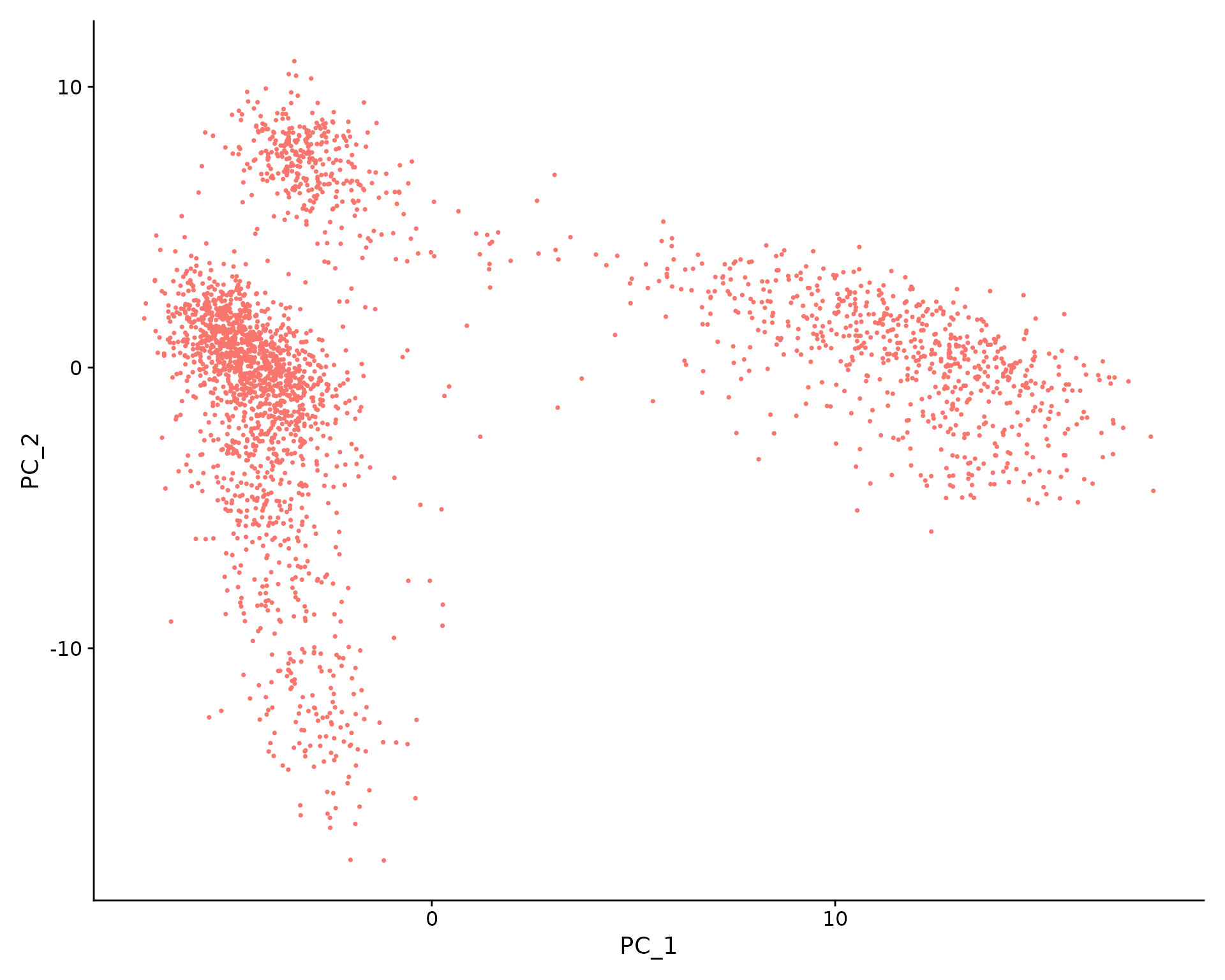
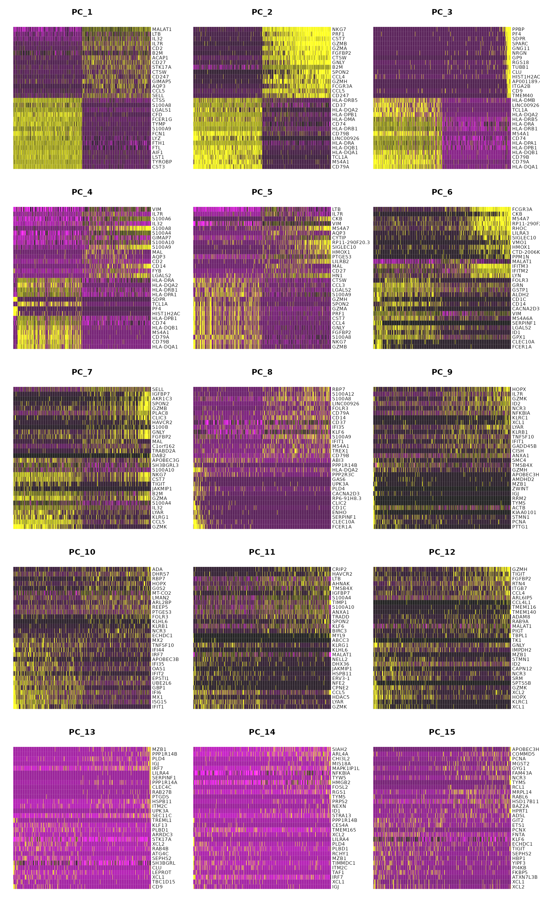
Perform linear dimensional reduction

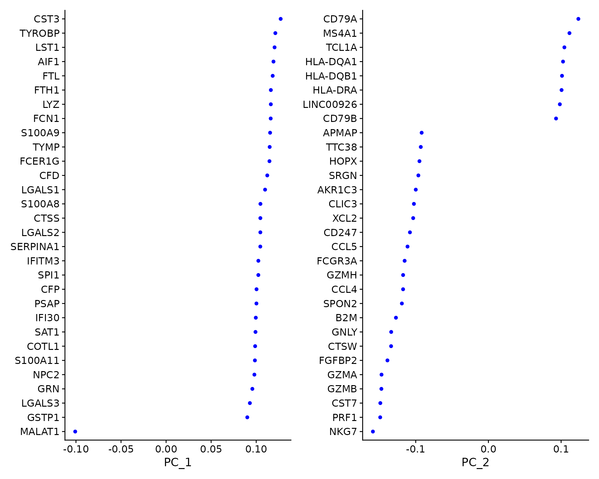
pbmc <- RunPCA(pbmc, features = VariableFeatures(object = pbmc))
# Examine and visualize PCA results a few different ways
print(pbmc[["pca"]], dims = 1:5, nfeatures = 5)
VizDimLoadings(pbmc, dims = 1:2, reduction = "pca")
Violine plot for QC
©Seurat 2021
DimPlot(pbmc, reduction = "pca")
Violine plot for QC
©Seurat 2021
DimHeatmap(pbmc, dims = 1:15, cells = 500, balanced = TRUE)
Violine plot for QC
©Seurat 2021

Determine the ‘dimensionality’ of the dataset

# NOTE: This process can take a long time for big datasets, comment out for expediency. More
# approximate techniques such as those implemented in ElbowPlot() can be used to reduce
# computation time
pbmc <- JackStraw(pbmc, num.replicate = 100)
pbmc <- ScoreJackStraw(pbmc, dims = 1:20)
JackStrawPlot(pbmc, dims = 1:15)
Violine plot for QC
©Seurat 2021
ElbowPlot(pbmc)
Violine plot for QC
©Seurat 2021

Cluster the cells

pbmc <- FindNeighbors(pbmc, dims = 1:10)
pbmc <- FindClusters(pbmc, resolution = 0.5)

# Look at cluster IDs of the first 5 cells
head(Idents(pbmc), 5)

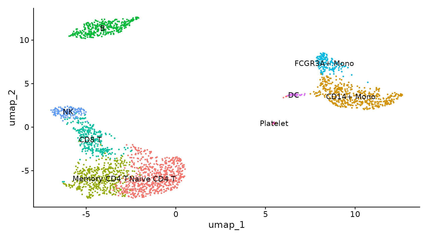
Run non-linear dimensional reduction (UMAP/tSNE)

# If you haven't installed UMAP, you can do so via reticulate::py_install(packages =
# 'umap-learn')
pbmc <- RunUMAP(pbmc, dims = 1:10)
DimPlot(pbmc, reduction = "umap")
saveRDS(pbmc, file = "../output/pbmc_tutorial.rds")
Violine plot for QC
©Seurat 2021

Finding differentially expressed features (cluster biomarkers)

cluster2.markers <- FindMarkers(pbmc, ident.1 = 2, min.pct = 0.25)
head(cluster2.markers, n = 5)

# find all markers distinguishing cluster 5 from clusters 0 and 3
cluster5.markers <- FindMarkers(pbmc, ident.1 = 5, ident.2 = c(0, 3), min.pct = 0.25)
head(cluster5.markers, n = 5)

pbmc.markers <- FindAllMarkers(pbmc, only.pos = TRUE, min.pct = 0.25, logfc.threshold = 0.25)
pbmc.markers %>%
group_by(cluster) %>%
slice_max(n = 2, order_by = avg_log2FC)

cluster0.markers <- FindMarkers(pbmc, ident.1 = 0, logfc.threshold = 0.25, test.use = "roc", only.pos = TRUE)
VlnPlot(pbmc, features = c("MS4A1", "CD79A"))
Violine plot for QC
©Seurat 2021
# you can plot raw counts as well
VlnPlot(pbmc, features = c("NKG7", "PF4"), slot = "counts", log = TRUE)
Violine plot for QC
©Seurat 2021
FeaturePlot(pbmc, features = c("MS4A1", "GNLY", "CD3E", "CD14", "FCER1A", "FCGR3A", "LYZ", "PPBP",
"CD8A"))
Violine plot for QC
©Seurat 2021
pbmc.markers %>%
group_by(cluster) %>%
top_n(n = 10, wt = avg_log2FC) -> top10
DoHeatmap(pbmc, features = top10$gene) + NoLegend()
Violine plot for QC
©Seurat 2021

Assigning cell type identity to clusters

new.cluster.ids <- c("Naive CD4 T", "CD14+ Mono", "Memory CD4 T", "B", "CD8 T", "FCGR3A+ Mono",
"NK", "DC", "Platelet")
names(new.cluster.ids) <- levels(pbmc)
pbmc <- RenameIdents(pbmc, new.cluster.ids)
DimPlot(pbmc, reduction = "umap", label = TRUE, pt.size = 0.5) + NoLegend()
saveRDS(pbmc, file = "../output/pbmc3k_final.rds")
Violine plot for QC
©Seurat 2021
Author

Karobben

Posted on

2021-10-30

Updated on

2024-01-22

Licensed under

Comments