Unsupervised Machine Learning in Python (DBSCAN; UMAP, t-SNE, etc)

DBSCAN

video instroctrions:

• Machine Learning TV: DBSCAN: Part 1; 2019; Youtube
• Machine Learning TV: DBSCAN: Part 1; 2019; Youtube
• Machine Learning TV: DBSCAN: Part 2; 2019; Youtube

Blog and Papers:

• Li, X.; Zhang, P.; Zhu, G. DBSCAN Clustering Algorithms for Non-Uniform Density Data and Its Application in Urban Rail Passenger Aggregation Distribution. Energies 2019, 12, 3722. https://doi.org/10.3390/en12193722
• Kelvin Salton do Prado: How DBSCAN works and why should we use it?; 2017

The ideas of DBscan

© Li, X, et al

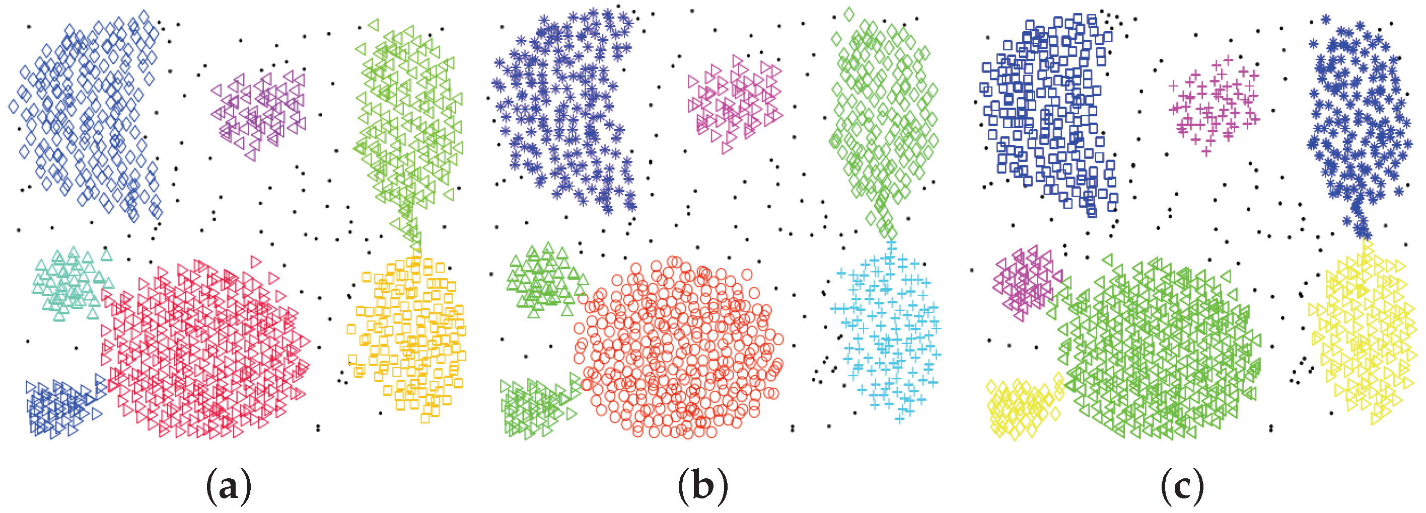
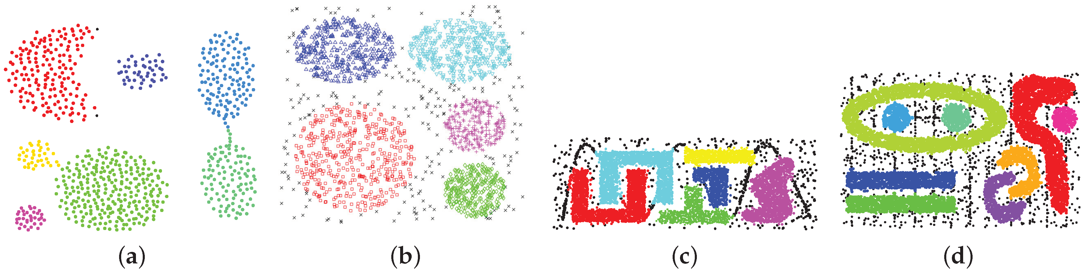
DBscan is cluster a group of nodes by the spatial distribution density.
It divided the nodes to “core point”; “border point”, and “outlier point”
By given the pre-assigned diameters (of the sphere) and number of the adjacent nodes, it scan the nodes randomly.

• The node fit our expectation is core node.
• The node failed to achieve the expectation but adjacent to the core point(a) is border point.
• Rest of nodes are outlier points

The advantage of DBscan is

• Outlier points (Noises) is tolerated. (Unlike k-means)
• It can detect the cluster under a cluster. (Not like spherical-shape cluster)

DNscan in python

Source codes: sklearn

from sklearn.cluster import DBSCAN
import numpy as np
X = np.array([[1, 2], [2, 2], [2, 3],
      [8, 7], [8, 8], [25, 80]])
clustering = DBSCAN(eps=3, min_samples=2).fit(X)
clustering.labels_
array([ 0,  0,  0,  1,  1, -1])
clustering

DBSCAN(eps=3, min_samples=2)

More examples: from SKlearn

UMAP

from umap import UMAP
import plotly.express as px


features = np.array(df)

umap_2d = UMAP(n_components=2, init='random', random_state=0)
umap_3d = UMAP(n_components=3, init='random', random_state=0)

proj_2d = umap_2d.fit_transform(features)
proj_3d = umap_3d.fit_transform(features)

t-SNE

from sklearn.manifold import TSNE
import plotly.express as px

features # pd.DataFram or np array

tsne = TSNE(n_components=2, random_state=0)
projections = tsne.fit_transform(features)

fig = px.scatter(
    projections, x=0, y=1,
    color=Cell_index.Group, #labels={'color': 'species'}
)
fig.update_layout({"plot_bgcolor": 'rgba(0, 0, 0, 0)'})
fig.show()

K-Means

from sklearn.cluster import KMeans

features # pd.DataFram or np array

kmeans = KMeans(n_clusters=15, random_state=0).fit(features)

print(kmeans.labels_)

Affinity Propagations

Youtube Tutorial: Soheil Behnezhad; 2017

source:scikit-learn.org
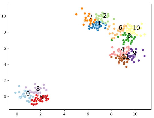
preferencearray-like of shape (n_samples,) or float, default=None

• Preferences for each point - points with larger values of preferences are more likely to be chosen as exemplars. The number of exemplars, ie of clusters, is influenced by the input preferences value. If the preferences are not passed as arguments, they will be set to the median of the input similarities.

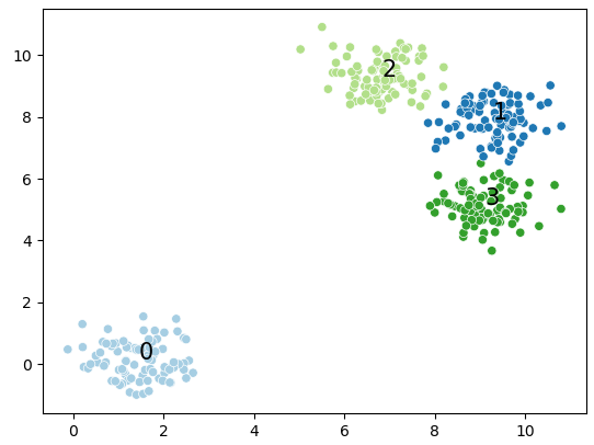
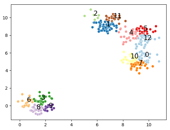
import numpy as np
import seaborn as sns
from sklearn.datasets import make_blobs
import matplotlib.pyplot as plt
from sklearn.cluster import AffinityPropagation

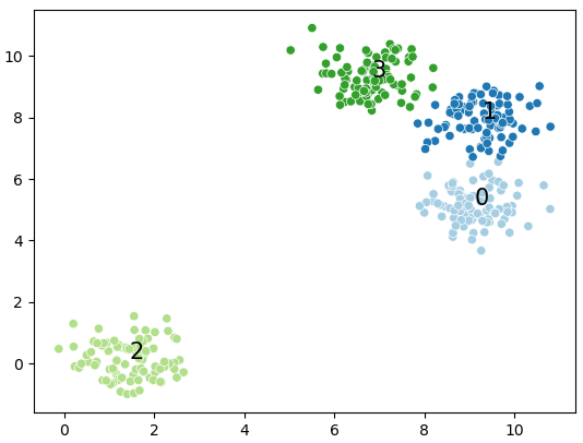
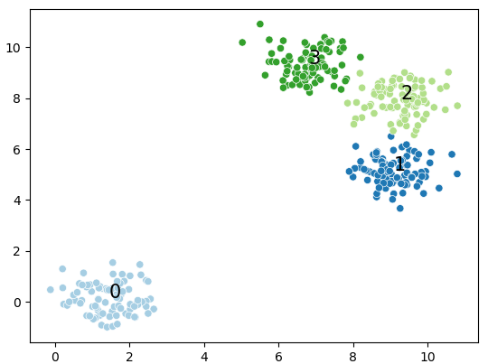
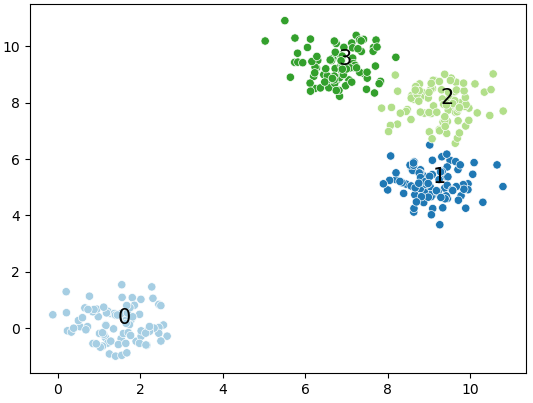
X, y = make_blobs(n_samples=350, centers=4, cluster_std=0.60)


afprop  = AffinityPropagation(preference=-15)
afprop.fit(X)
labels = afprop.predict(X)

sns.scatterplot(x=X[:,0], y=X[:,1], hue= labels, legend=None,
 palette="Paired")
for i in set(labels):
  TMP = X[labels ==i]
  plt.text(x=TMP.mean(axis=0)[0], y=TMP.mean(axis=0)[1],
    s=str(i), size = 15)

plt.show()

preference=-15	preference=-99

MeanShift

import numpy as np
import seaborn as sns
from sklearn.datasets import make_blobs
import matplotlib.pyplot as plt
from sklearn.cluster import MeanShift

clustering = MeanShift(bandwidth=.6).fit(X)
labels = clustering.labels_

sns.scatterplot(x=X[:,0], y=X[:,1], hue= labels, legend=None,
 palette="Paired")
for i in set(labels):
  TMP = X[labels ==i]
  plt.text(x=TMP.mean(axis=0)[0], y=TMP.mean(axis=0)[1],
    s=str(i), size = 15)

plt.show()

bandwidth=.6	bandwidth=1

Spectral Clustering

from sklearn.cluster import SpectralClustering

sc = SpectralClustering(n_clusters=4).fit(X)
labels = sc.labels_

sns.scatterplot(x=X[:,0], y=X[:,1], hue= labels, legend=None,
 palette="Paired")
for i in set(labels):
  TMP = X[labels ==i]
  plt.text(x=TMP.mean(axis=0)[0], y=TMP.mean(axis=0)[1],
    s=str(i), size = 15)

plt.show()

n_clusters=13	n_clusters=4

OPTICS cluster

from sklearn.cluster import OPTICS

clustering = OPTICS(min_samples=1, min_cluster_size=13).fit(X)
label = clustering.labels_

sns.scatterplot(x=X[:,0], y=X[:,1], hue= labels, legend=None,
 palette="Paired")
for i in set(labels):
  TMP = X[labels ==i]
  plt.text(x=TMP.mean(axis=0)[0], y=TMP.mean(axis=0)[1],
    s=str(i), size = 15)

plt.show()

Hierarchy

Reference:

• Jörn’s Blog; 2016; SciPy Hierarchical Clustering and Dendrogram Tutorial
• coradek; 2018; Display cluster labels for a scipy dendrogram

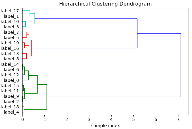
from scipy.cluster.hierarchy import dendrogram, linkage
import scipy.stats as stats
from scipy.cluster.hierarchy import cophenet
from scipy.spatial.distance import pdist
from sklearn.datasets import make_blobs


X, y = make_blobs(n_samples=350, centers=4, cluster_std=0.60)
XX= X[:20]

Z = linkage(stats.zscore(XX) , 'ward')
c, coph_dists = cophenet(Z, pdist(XX))
label = ["label_" + str(i) for i in range(len(XX))]

temp = {ii: label[ii] for ii in range(len(label))}
def llf(xx):
    return temp[xx]

Z = linkage(stats.zscore(XX) , 'ward')

plt.title('Hierarchical Clustering Dendrogram')
plt.xlabel('sample index')
plt.ylabel('distance')
dendrogram(
    Z,
    orientation='right',
    leaf_label_func=llf,
    leaf_rotation=0.,  # rotates the x axis labels
    leaf_font_size=10.,  # font size for the x axis labels
)
plt.show()