BioStatistics with R/Python: Block 2

Biomedical Statistics and Data Analysis: Block 2

L8: Counted Variables and Their Asymmetric Distributions

What is Sample count? Count Variable

• For an event to be counted it has to occur AND it has to be observed.
• Counted variables are treated differently than measured variables because their distributions are asymmetric (not Gaussian). (use binomial statistics)
• To be able to apply the statistical treatments that we will use, the counted events must follow the following rules:
  • Each event has a probability of occurring or a random probability of being observed (or both).
  • Occurrence or observation (or both) is a random event.
  • The probability of occurrence/observation is independent of whether other occurrences/observations have been made.
• If both the occurrence of an event and its observation are non random or known with certainty then the statistical principles related to counted variables do not apply.

Examples

• Examples of counted variables where the occurrence is random but the observation is certain:
  • Proportion of planes that crash
  • Number of cars that drive past a certain intersection
  • Number of patients that die when treated with a drug
• Examples of counted variables where the occurrence is certain but the observation is random:
  • Number of turtles counted in a lake
  • Radioisotope concentration
• Examples of counted variables where both occurrence and observation is random:
  • Number of people with the flu
  • Number of cells that are transfected
• Examples of counted variables where neither the occurrence nor the observation is random:
  • The number of turtles in a bathtub
  • The number of toes on your left foot
  • The number of presidents with wives named “Barbara”

Question: Are you categorizing or just counting events (or categorizing)?

If you are categorizing events (yes/no, live/dead, success/failure, democrat/republican) use binomial statistics. INSTAT does not deal with single proportions very well. OS4 and SSP will use do calculations for proportions. SSP uses the word “probability” to denote proportions.

If you are counting events Car crashes, weddings in July, deaths
from lung cancer, radioactive counts) use Poisson statistics.

Binomial DIstribution

$$
P_ {x:n} = \frac{n!}{x!(n-x)!} p^x (1-p)^{n-x}
$$

• $\frac{n!}{x!(n-x)!}$:
  Of combinations (how many different ways are there of doing an experiment)
• $p^x$:
  Probability of x Successes in one experiment.
• $(1-p)^{n-x}$:
  Probability of n-x failures in one experiment (n trials).

# Do it yourself
Bi_cal <- function(x, n, p){
  R = ncol(combn(n,x)) * (p^x) * ((1-p)^(n-x))
  return (R)
}

# From R default functions
dbinom(4, size=12, prob=0.2)

Exp: Probability of getting 2 heads when flipping 3 coins = 3 x 0.25 x 0.5 = 0.375
in r:
dbinom(2, size=3, prob=0.5)

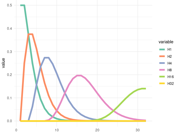
Codes for the Graphic

library(ggplot2)
library(reshape2)
x= c(1:32)
Pro = data.frame(x=x, H1 = dbinom(1, size=x, prob=0.5),
  H2 = dbinom(2, size=x, prob=0.5),
  H4 = dbinom(4, size=x, prob=0.5),
  H8 = dbinom(8, size=x, prob=0.5),
  H16 = dbinom(16, size=x, prob=0.5),
  H32 = dbinom(32, size=x, prob=0.5)
)

Pro_TB = melt(Pro, id.vars = 'x')

ggplot(Pro_TB, aes(x= x, y =value, group = variable, color=variable)) +
  geom_line(size= 2)+ theme_minimal()+
  scale_color_brewer(palette = "Set2")

The H1 means the chase for get 1 head in times of rolled at x. So as the H2, 4, 8, 16, and 32

The binomial distribution is used to describe small numbers of discreet events, or proportions of small numbers. Becomes a Gaussian distribution as n gets large. Mean and standard deviation of the parent distribution can be calculated.

$μ= np$

• μ is the mean number of “successes”, n is the number of trials
• p is the probability of success in each trial
• $σ_ μ = \sqrt{np(1-p)}$
• The standard deviation in μ (# successes)

If p is not known it must be estimated from the
data. p is successes divided by total i.e. (μ/n)

Data that would use a Binomial Distribution

Example: You know that normally 1 person in 8 has a negative reaction to a particular drug.
1. How many negative reactions would you expect to have in a sample of 21 people?

In this questions, we can know that the p = 1/8
So, we can have $\mu = np= 21\times (1/8) = 2.63$
We supposed have 2.63 people is negative
And then: $\sigma = \sqrt{np(1-p)}= \sqrt{21 × (1/8)(7/8)} = 1.52$ The SD is 1.52
2. What is the probability of observing zero negative reactions in 21 patients?
dbinom(0, 21, 1/8)

[1] 0.06055766

Example: You conducted a random phone poll of 900 people and found that 45% favored candidate A and 55% favored candidate B.
What is the uncertainty of the result (What is the standard deviation?).
This question is actually calling for the relative uncertainty. which is μ/σ
$µ=np=900×.45= 405$
$\sigma = \sqrt{np(1-p)}=\sqrt{900×0.45(1-0.45)}=14.92481$
Relative uncertainty = μ/σ = 3.7%

The Poisson Distribution

When p « 1 or when n » x the binomial distribution simplifies to the Poisson distribution. The Poisson distribution also applies when you are counting discreet events (presumably from a very large population of possible observations) but not categorizing them as successes/failures or left/right or alive/dead or sick/not sick.

$$
p = \frac{\mu^ x}{x!}e^{-\mu}
$$

$\mu=np=x$
$\sigma = \sqrt{np(1-p)}$;
When the p « 1, we then have: $σ = \sqrt{np}= \sqrt{x}$

The standard deviation of a counted variable is the square root of the # of counts. Ex: Political polls, radioactive counts, cell counts etc

Special case:
If the probability of seeing an event is 1/n and you try n times, the probability of seeing the event once is only 37%. This is exactly the same as the probability of not seeing the event at all. There is a 63% chance is seeing it at least once.

Binomial versus Poisson Statistics: Which do we use?

Finally: The binomial equation is used when counting ratios or proportions of small numbers ( i.e. n/m where n< 100, n<m and m<100).
If we were counting the number cars that drive up to an intersection, that would be described with a Poisson distribution. While counting the number that turn left relative to the total would normally be described with a binomial distribution.

The binomial equation is used when categorizing. In other words, when your data are ratios or proportions of counted variables.

The Poisson equation is used when counting only and not categorizing.

When the numerator of a ratio is very large, the binomial and Poission descriptions become equivalent.

Examples:

• If we were counting the number cars that pass a certain intersection, that would be described with a Poisson distribution, because it is a simple count.
• If we are counting the number of cars that hat turn left and the number that turn right, that would be described with a binomial distribution because it is a categorization.
• Assume you are doing yeast genetic studies and are counting the number of transformed colonies.
• If the transformation is frequent, you can plate a small number of colonies (<1000), count transformed and normal colonies, and analyze the statistics using proportions (binomial).
• If the transformation is rare, you can plate thousands of colonies, count only the transformed colonies and analkyze the statistics using simple counts (Poisson).

L9: Confidence intervals for proportions and counts

How to determine statistical significance of one proportion versus a null hypothesis:

1. Determine the upper and lower bounds of the confidence interval. Use 1-α for probability. 95% CI for α=0.05.
2. Compare H0 to the CI. If Ho is inside the CI, the difference is not significant. If H0 is outside the CI, the difference IS significant.

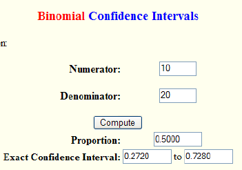
How to calculate the 95% confidence Intervals.

R codes: Wayne W. LaMorte, MD, PhD, MPH

prop.test(10,20,p=.5)

  1-sample proportions test without continuity correction

  data:  10 out of 20, null probability 0.5
  X-squared = 0, df = 1, p-value = 1
  alternative hypothesis: true p is not equal to 0.5
  95 percent confidence interval:
  0.299298 0.700702
  sample estimates:
  p
  0.5

library(Hmisc)
#calculate 95% confidence interval
binconf(x=10, n=20, alpha=.05)

  PointEst    Lower    Upper
     0.5 0.299298 0.700702

Results from Exact Binomial and Poisson Confidence Intervals :

Special case for a proportion:

How do you determine p-value when the Null hypothesis is 0 or 1?

There is a problem we have to solve:

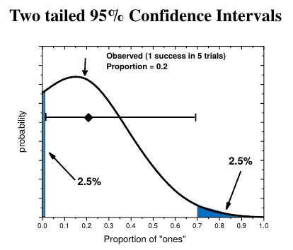
• The exact two-sided CI (by definition) can never include a proportion of 0 or 1 (because we are forcing it to have equal area on each side).

Yet, in some cases the probability of observing a proportion of exactly zero 0 or 1 will be greater than 0.025 (half of the 95% CI) and thus should not be considered significant.

How do we decide if a null hypothesis proportion of 0 or 1 is really statistically different from a experimentally derived proportion? There are two approaches.

1. Exact Solution: Go to a binomial probability calculator and calculate the probability for x=0 (or x=n) for your proportion. If p>0.025 then the limit (proportion = 0 or 1) should be considered WITHIN the CI and not significantly different.

2. Approximate solution (works well for trials > 10): Determine the 2 sided CI of your proportion. If the 1/n is within the CI, then a proportion of 0 is NOT statistically significant. If (x-1)/x is within the CI then a proportion of 1 is NOT statistically significant.

HINT: For any experiment with at least 12 trials, if the successes = 3 or less, it will not be statistically different from a proportion of zero.
Similarly, if the number of trials is 12 or more and trials-successes = 3 or less, it will never be significantly different from a proportion of 1.

Example: You measured a proportion of 3/15. Is there a statistically significant difference from a Null hypothesis proportion = 0?
Using the statpages site or table above the CI of the proportion 3/15 is 0.043 – 0.481.

1. Exact method: Using a binomial calculator (above) with N=15 and prop = 0.2 (3/15), the probability of x=0 is 0.0352. Since this is larger than the one-tailed probability of 0.025 (for =0.05) it is NOT significant.
2. Approximate Method: The value 1/n or 1/15 is 0.067. Since this value falls within the CI 0.043-0.481, a proportion of 0 is NOT significantly different from your measured 3/15.

So, after interpretation from above, we now know that we’d like to know the difference between 3/15 and 0/15. So, the code in R could be: prop.test(0,15, p = 3/15)

1-sample proportions test with continuity correction
data:  0 out of 15, null probability 3/15
X-squared = 2.6042, df = 1, p-value = 0.1066
alternative hypothesis: true p is not equal to 0.2
95 percent confidence interval:
0.0000000 0.2534679
sample estimates:
p
0

p-value = 0.1066, which means is not significantly different. The null hypothesis is accepted and 3/15 has no difference from 0/15.

Confidence Interval of a Poisson distributed (counted) value

How do you determine statistical significance for the null hypothesis that a
proportion equals a certain value?

• A 95% CI is equal to p- value of 0.05. Calculate a CI for the proportion using one of the methods we just discussed. If CI includes the null hypothesis, then p is larger than your cutoff (thus not significant). If the CI does not include the null hypothesis p is smaller and is significant.

Example:
Suppose you observed 5 mice out of 30 transgenic mouse offspring were male. You wanted to know if there was a gender specific mortality effect. Your null hypothesis is 0.5 (half male, half female). Observed Ratio = 0.17 95% CI = 0.056-0.347 (From Table) Since the 95% CI does not include Null hypothesis, p is smaller than 0.05 and is significant.

In r, We know that the observe is 5, sample size is 30, and expectation is 0.5. So, we can have:

prop.test(5,30,.5)

1-sample proportions test with continuity correction
data:  5 out of 30, null probability 0.5
X-squared = 12.033, df = 1, p-value = 0.0005226
alternative hypothesis: true p is not equal to 0.5
95 percent confidence interval:
 0.06303555 0.35451084
sample estimates:
        p
0.1666667

We can see that the p = 0.0005226, which means the result is significant.

Example: Poisson Confidence Intervals
A newspaper headline proclaims that the roads in Southern Louisiana have become less safe in 2004 because the 138 fatal accidents that year was 11% higher than the long term average number of 124 per year. Use statistics to analyze this conclusion. Are the roads more dangerous?

Since 124 is a long term average we use it in this simple example as a null hypothesis without uncertainty.
In r, we just need use: poisson.test(138)

       Exact Poisson test
data:  138 time base: 1
number of events = 138, time base = 1, p-value < 2.2e-16
alternative hypothesis: true event rate is not equal to 1
95 percent confidence interval:
  115.9369 163.0397
sample estimates:
event rate
       138

We can see that the confidence interval is from 115.9369 to 163.0397. And 115.9369 < 124 < 163.0397. So, the result is not significant difference.

More examples for understanding

Example 1: If your data are the proportion of dead cells on a plate and you measured in each of four fields: 31/120; 18/56; 40/103; 44/121

• You recalculate your total proportion as (31+18+40+44) / (120+56+103+121) or 133/400.
• We use 1-sample proportions: prop.test(133, 400)
• the CI: 0.2869229 0.3813495
• the proportion of 4 experiments are: 0.2583333, 0.3214286, 0.3883495, 0.3636364. The first experiment is significantly different from others.

Example 2: Your Geiger counter reports counts in 1 minute intervals: 12,15,8,17,12,11,9 and 13 Your confidence interval is based on total counts = 97 (12.1 cpm)
poisson.test(97) tell us that the CI is: 78.66047 118.33177, which means it’s 9.832558 14.791472 per minute. We can find that the 8 and 9 is the outlier.

L10: Contingency Tables

• It is used in statistics to summarize the relationship between several categorical variables. A contingency table is a special type of frequency distribution table, where two variables are shown simultaneously.
• Instruction in Excel

Clinical studies sometimes use a binary (yes/no) decision to assess disease or outcome. So clinical studies are often analyzed as a proportion of a counted variable. There are four main types of clinical studies:

• Retrospective (case-control): Start with outcome (e.g. disease) and look back to see the cause with cases (disease) and controls (no disease).
• Prospective: Start with exposure and follow cases to see if disease develops. Also uses cases (exposed or hypothetical risk factor) and controls (not exposed, or no hypothetical risk factor).
• Cross-sectional: Start with a set of randomly selected subjects that are NOT selected based disease or exposure. Divide into two groups and assess the correlation between disease and hypothetical risk factor.
• Experimental: Randomly selected subjects, Split into two groups, subject one groups to a treatment, the other to a control treatment such as a placebo.

Find the correlated with the diseases.

Exp1: How you compare multiple proportions with one another?

Imagine a small scale experimental cancer drug trial. You recruit 40 patients with end-stage cancer. 20 get drug and 8 of them survive 5 years. Another 20 get placebo and 2 of them survive 5 years.

contingency table

	Survival	Not Survival
Treated	8	12
Not Treated	2	18

Codes for R: December 19, 2020 by George Pipis in R bloggers

TB2 <- data.frame( Survival = c(8, 2),
          Dead=c(12, 18),
          row.names = c("Treated", "Placebo"))

prop.table(TB2)
chisq.test(TB2)
fisher.test(TB2)

  Survival Dead
  Treated     0.20 0.30
  Placebo     0.05 0.45

  Pearson's Chi-squared test with Yates' continuity correction

  data:  TB2
  X-squared = 3.3333, df = 1, p-value = 0.06789

  Fisher's Exact Test for Count Data

  data:  TB2
  p-value = 0.06483
  alternative hypothesis: true odds ratio is not equal to 1
  95 percent confidence interval:
  0.9222194 64.6794654
  sample estimates:
  odds ratio
  5.735024

We can see that P value from both Chi-squared test and Fisher’s Exact test are larger than 0.05, which means the null hypothesis is accepted and they have no significant difference.

Exp 2: An example of a clinical trial with a single outcome

Suppose you are performing an experimental study to determine if AZT improves the outcome of HIV-infected patients. All patients are infected with HIV, some are treated with AZT some with placebo. You determine which patients develop clinical symptoms of AIDS and which do not. Disease developed in 28% of placebo-treated cases (129/461) and in 16% of AZT treated cases (76/475).

	AIDS	No AIDS	Total
ATZ	76(TD)	399(TN)	475(Tx)
Placebo	129(ND)	332(NN)	461(Nx)
Total	205(xD)	731(xN)	936

TB <- data.frame( AIDS = c(76, 399),
          N_AIDS=c(129, 332),
          row.names = c("AZT", "Placebo"))

prop.table(TB)
chisq.test(TB)
fisher.test(TB)

  AIDS    N_AIDS
  AZT     0.08119658 0.1378205
  Placebo 0.42628205 0.3547009

  Pearson's Chi-squared test with Yates' continuity correction

  data:  TB
  X-squared = 18.944, df = 1, p-value = 1.346e-05

  Fisher's Exact Test for Count Data

  data:  TB
  p-value = 9.24e-06
  alternative hypothesis: true odds ratio is not equal to 1
  95 percent confidence interval:
  0.3512693 0.6818650
  sample estimates:
  odds ratio
  0.4905877

P value is signifcant and so, the H₀ hypothesis is rejected and the drug works.

Explained:
If you want to measure the confidence interval for the difference between the proportions. You can do it with a Gaussian approximation if none of the entries are smaller than 5 and none of the same-row values are within 5 of each other. (In other words, if neither proportion is close to zero or close to 1.0).

$$
CI = (p_ 1 - p_ 2) ± z × \sqrt{\frac{p_ 1 (1-p_ 1)}{n_ 1} + \frac{p_ 2 (1-p_ 2)}{n_ 2}}
$$

Other ways of expressing proportional results:

• Relative risk(RR)
  $$
  RR = \frac{p_ 1}{p_ 2}
  $$

Relative risk is sometimes called relative rate or relative probability, especially in non-clinical studies. Pay attention to which outcome is in the numerator (on top).
In the AZT study, the relative risk is 0.57. AZT patients were 57% as likely as placebo patients to have disease progression. If we switched places of the two treatments (which would be perfectly valid) we would be saying that placebo patients were 1.75 time as likely to have disease progression.

• Number Needed to Treat
  $$
  NNT = \frac{1}{(p_ 2 - p_ 1)}
  $$

• Odds ratio (OR)
  $$
  OR = (\frac{Odds_ 1}{Odds_ 2}= \frac{TD/TN}{ND/NN})
  $$

Exp 3

Cat scratch fever is a mild disease that is transmitted by cats. A case-control study assessed whether there is an connection between fleas and the disease in humans. (That is fleas on the cats and disease in the humans).

	Disease	No Disease	Total
Fleas	32(TD)	4(TN)	36(Tx)
No Fleas	24(ND)	52(NN)	76(Nx)
Total	56(xD)	56(xN)	112

TB <- data.frame( Disease = c(32, 4),
          N_Disease=c(24, 52),
          row.names = c("Fleas", "N_Fleas"))

prop.table(TB)
chisq.test(TB)
fisher.test(TB)

  Disease N_Disease
  Fleas   0.28571429 0.2142857
  N_Fleas 0.03571429 0.4642857

  Pearson's Chi-squared test with Yates' continuity correction

  data:  TB
  X-squared = 29.842, df = 1, p-value = 4.687e-08

  Fisher's Exact Test for Count Data

  data:  TB
  p-value = 1.201e-08
  alternative hypothesis: true odds ratio is not equal to 1
  95 percent confidence interval:
  5.171911 72.958931
  sample estimates:
  odds ratio
  16.84407

According to Fisher’s Extrac test, the CI is 5.171911 to 72.958931, which means that cat owners with fleas (cat owners whose cats have fleas) are between 5 and 73 times more likely to get cat scratch fever as cat owners whose cats do not have fleas.

Contingency table in R

Exp1: Łukasz Deryło, 2018

# Practice 1
library(MASS)
#check the observes by yourselves
#Cars93$Type
table(Cars93$Type)
prop.table(table(Cars93$Type))

# Practice 2
table(Cars93$Origin)
prop.table(table(Cars93$Origin))

# How to make a contingency table
table(Cars93$Type, Cars93$Origin)

• Practice 1:
  

  
  
  Compact   Large Midsize   Small  Sporty     Van
  
  16      11      22      21      14       9
  
  Compact      Large    Midsize      Small     Sporty        Van
  
  0.17204301 0.11827957 0.23655914 0.22580645 0.15053763 0.09677419
  
  

• Practice 2:

USA non-USA
48      45

USA  non-USA
0.516129 0.483871

• How to make a contingency table

USA non-USA
Compact   7       9
Large    11       0
Midsize  10      12
Small     7      14
Sporty    8       6
Van       5       4

After probability

• Fisher’s exact test

fisher.test(Cars93$Type, Cars93$Origin)

Fisher's Exact Test for Count Data
#
data:  Cars93$Type and Cars93$Origin
p-value = 0.007248
alternative hypothesis: two.sided

• G-test

library(DescTools)
GTest(Cars93$Type, Cars93$Origin)

Log likelihood ratio (G-test) test of independence without correction
#
data:  Cars93$Type and Cars93$Origin
G = 18.362, X-squared df = 5, p-value = 0.002526

• Yates’ correction

chisq.test(table(Cars93$Man.trans.avail, Cars93$Origin))

Pearson's Chi-squared test with Yates' continuity correction
#
data:  table(Cars93$Man.trans.avail, Cars93$Origin)
X-squared = 15.397, df = 1, p-value = 8.712e-05

• 3 (or more) dimensional table

table(Cars93$Man.trans.avail, Cars93$Origin, Cars93$Type)

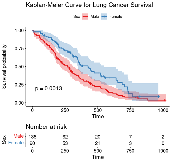
L12: Survival Curve

Targets for Survival Curve

• Plot Kaplan-Meier Curve
• P-value: Log-rank (Mantel-Cox) test and Gehan-Breslow-Wilcoxon test (which has more weight to early events)
• Hazard Ratio: Mental-Haenszel and logrank

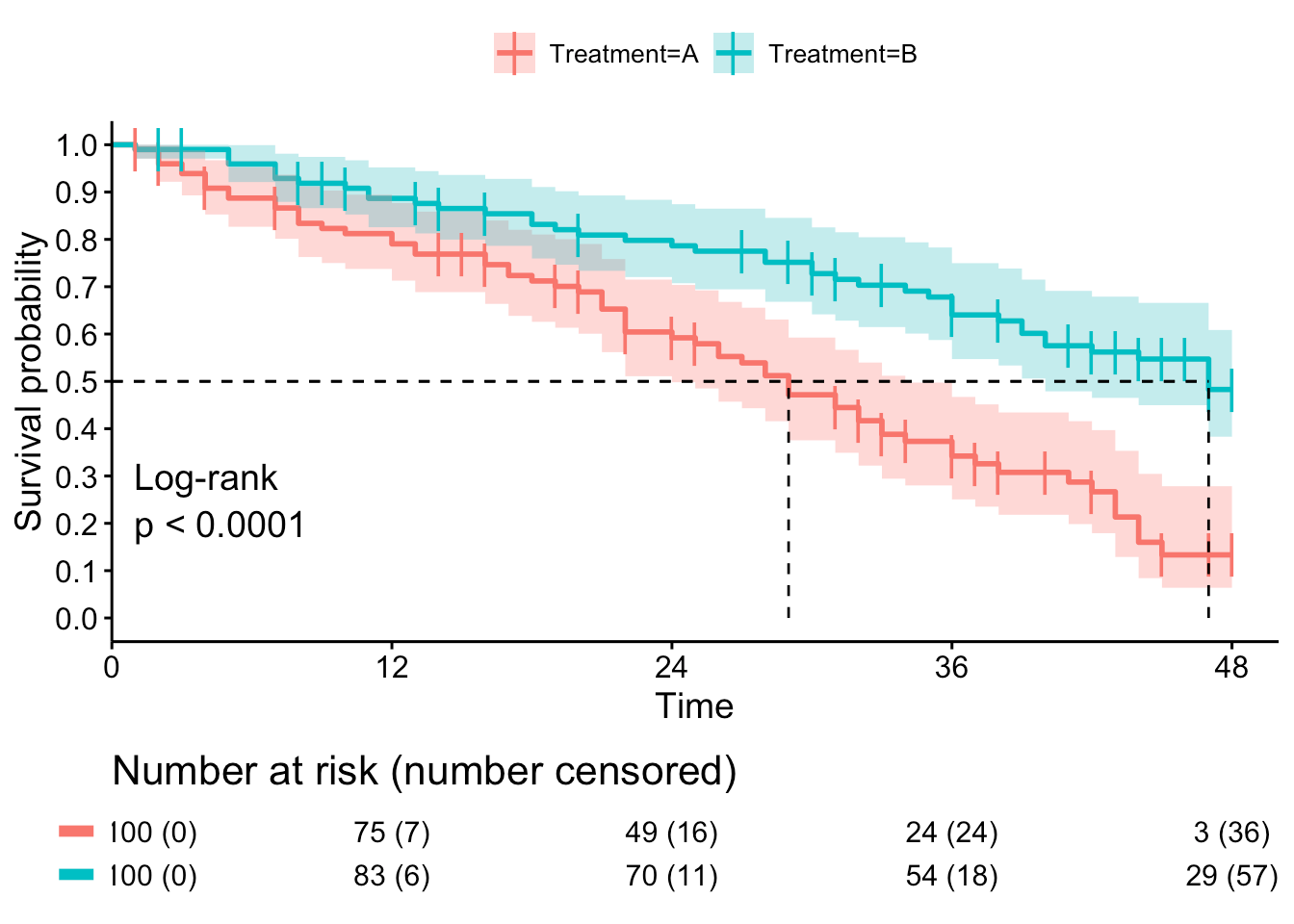
Kaplan-Meier Curve

• Plots percent survival of each cohort relative to non-censored totals.
• A tic mark indicates a censoring event.

© Ruben Van Paemel; 2019

Online Calculator: evanmiller.org

R in action

Quick start with survival package
More detailed examples and codes: bioconnector
The most informative and detailed posts: Emily C. Zabor

Practive Data:

library(survival)
?lung

  inst:       Institution code
  time:       Survival time in days
  status:     censoring status 1=censored, 2=dead
  age:        Age in years
  sex:        Male=1 Female=2
  ph.ecog:    ECOG performance score as rated by the physician.
              0=asymptomatic, 1= symptomatic but completely ambulatory, 2= in bed
              <50% of the day, 3= in bed > 50% of the day but not bedbound, 4 =
              bedbound
  ph.karno:   Karnofsky performance score (bad=0-good=100) rated by physician
  pat.karno:  Karnofsky performance score as rated by patient
  meal.cal:   Calories consumed at meals
  wt.loss:    Weight loss in last six months

The data we need is in time, Survival time in days, and status, Censored or dead

library(survival)
library(survminer)

sfit <- survfit(Surv(time, status)~sex, data=lung)
ggsurvplot(sfit, conf.int=TRUE, pval=TRUE, risk.table=TRUE,
           legend.labs=c("Male", "Female"), legend.title="Sex",  
           palette="Set1",
           title="Kaplan-Meier Curve for Lung Cancer Survival",
           risk.table.height=.25)
fit <- coxph(Surv(time, status)~sex, data=lung)
fit

Call:
coxph(formula = Surv(time, status) ~ sex, data = lung)

       coef exp(coef) se(coef)      z       p
sex -0.5310    0.5880   0.1672 -3.176 0.00149

Likelihood ratio test=10.63  on 1 df, p=0.001111
n= 228, number of events= 165

L13: Power and Sample Size

The function power.t.test from R has the same result from Java applets for power and sample size, which is different from some others.

Example: You have measured 2.3±5.0 (SD, n=26) and determined that p=0.027 for H_o=0. What is the power of your experiment?

• Mean=2.3, H₀= 0, as a result, delta = 2.3-0 =2.3.
• Because the null hypothesis is 0, we only need the lesser side. So, we should use one.sample t test.
  In R, we can have: power.t.test(n = 40, delta = 2.3, sd = 5, type="one.sample", alternative = "two.sided")

One-sample t test power calculation

        n = 40
    delta = 2.3
       sd = 5
sig.level = 0.05
    power = 0.8097611
alternative = two.sided

We can tell that the power is 0.81, which means you got 80.98% of chance to have the significant result.

With the same data, if we’d like to improve the changes to 95%, than, we can have: power.t.test(power = .95, delta = 2.3, sd = 5, type="one.sample", alternativ = "two.sided")

One-sample t test power calculation

        n = 63.36733
    delta = 2.3
       sd = 5
sig.level = 0.05
    power = 0.95
alternative = two.sided

Now, we can know that we need at least 64 tests to get a significant result with the chance of 95% in success.

Example 1: In a preliminary experiment you measure 12±4 (SD). You want to estimate sample size required to detect a difference of ±0.5 (H_o – mean) with a power of 90%. The confidence level you will use is 95% (α=0.05)

Two-sample t test power calculation

        n = 1345.911
    delta = 0.5
       sd = 4
sig.level = 0.05
    power = 0.9
alternative = two.sided

Example 2: If around 10% of the population suffers from migraine headaches. How many people would you have to enroll in an experimental clinical study to determine if prophylactic daily aspirin use will reduce the number of people who have migraines to 8%. Your desired confidence level is 95% and the desired power is 50%.
power.prop.test(p1=.1, p2 = .08, power = .5)

Two-sample comparison of proportions power calculation

        n = 1573.077
       p1 = 0.1
       p2 = 0.08
sig.level = 0.05
    power = 0.5
alternative = two.sided

We know that with the power of 0.5, we need to at least have 1574 sample for each. So, for a test with control, we’d like to have at least 1574*2=3148 for the experiment.