Python: Cell masks result analysis

Image mask to data frame

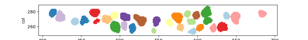
In this blog, I’ll show some tricks I used in cell marks processing. The data could be any kind of image or file. I am using CellPose to detect cells and get the mask. With this result, we can do quantification and size calculations. By comparing the raw image, we can also get the gray intensity or so.

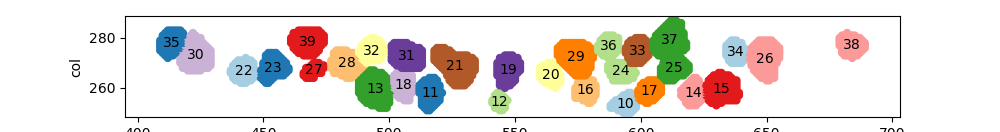
But of course, we are not just want to do the basic counts like that. We’d like to do more. In this post, I’ll show how to plot the cell based on the mask result, label the ID of each cell, calculate the Voronoi spacial, and finally determine the adjacent cells.

More related techniques would be updated if I had some new ideas and tasks.

RGB image

This code could turn your image to an pandas data frame. x and y would be list to the first two columns and color values would following.

IMG = cv.imread()

A = IMG
# Create the multiindex we'll need for the series
index = pd.MultiIndex.from_product(
    (*map(range, A.shape[:2]), ('r', 'g', 'b')),
    names=('col','row',  None)
)

# Can be chained but separated for use in explanation
df = pd.Series(A.flatten(), index=index)
df = df.unstack()
df = df.reset_index().reindex(columns=['row', 'col', 'r', 'g'. 'b'])

sns.scatterplot(data=df[df.r!=0], x= "row", y="col", hue = "r")
plt.show()

grey/mask fill

For CellPose, we can save the result as npy. Both raw image and mask results are saved in it. After read the npy file, we still need to convert them into DataFrame for further calculation.

import cv2
import pandas as pd
import numpy as np
import matplotlib.pyplot as plt
import seaborn as sns

NP_result = np.load("lgl.3d.casp.1.lsm2_seg.npy", allow_pickle=True)

A = NP_result.all()['masks']

# Create the multiindex we'll need for the series
index = pd.MultiIndex.from_product(
    (*map(range, A.shape[:2]), (['r'])),
    names=('col','row',  None)
)

# Can be chained but separated for use in explanation
df = pd.Series(A.flatten(), index=index)
df = df.unstack()
df = df.reset_index().reindex(columns=['row', 'col', 'r'])

sns.scatterplot(data=df[df.r!=0], x= "row", y="col", hue = "r")
plt.show()

Example data

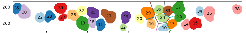
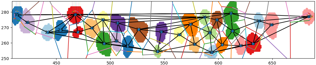
For save the time and have more detailed presentation, I only selected 30 cells to run the test which achieved very good results. I also applied this pipeline into the whole data and also in some other samples which also has thousands of cell and achieved very promising results.

df = df[df.r != 0]
df = df[df.r.isin(range(10,40))]

fig, ax = plt.subplots(figsize = ((df.row.max() - df.row.min())/28, (df.col.max() - df.col.min())/28))

sns.scatterplot(data=df, x= "row", y="col", hue = "r", linewidth = 0, palette= "Paired", legend = None )
fig.savefig("123.png")
plt.show()

Show labels of each cell

# calculate the position for each label
Label_TB = pd.DataFrame()
for ID in df.r.unique():
  TMP = df[df.r==ID]
  TMP_TB = pd.DataFrame(TMP.mean()).T
  Label_TB = pd.concat([Label_TB, pd.DataFrame(TMP.mean()).T])

Now, we can add the text into the cells

fig, ax = plt.subplots(figsize = ((df.row.max() - df.row.min())/28, (df.col.max() - df.col.min())/28))

sns.scatterplot(data=df, x= "row", y="col", hue = "r", linewidth = 0, palette= "Paired", legend = None )

for index in range(len(Label_TB)):
  plt.text(x= Label_TB.row.iloc[index],
  y=Label_TB.col.iloc[index],
  s= str(int(Label_TB.r.iloc[index])),
  horizontalalignment='center',
  verticalalignment='center',
)
#fig.savefig("123.png")
plt.show()

Delaunay triangulation to find adjacent cells

scipy.spatial.Delaunay

from scipy.spatial import Delaunay

Label_TB

points = Label_TB[['row', 'col']].to_numpy()
tri = Delaunay(points)


fig, ax = plt.subplots(figsize = ((df.row.max() - df.row.min())/28, (df.col.max() - df.col.min())/28))
sns.scatterplot(data=df, x= "row", y="col", hue = "r", linewidth = 0, palette= "Paired", legend = None )

plt.triplot(points[:,0], points[:,1], tri.simplices,color="white")
plt.plot(points[:,0], points[:,1], '.', color="black")
plt.show()

from collections import defaultdict
import itertools

neiList=defaultdict(set)
for p in tri.vertices:
    for i,j in itertools.combinations(p,2):
        neiList[i].add(j)
        neiList[j].add(i)

neiList

array([[593.98529412, 253.70588235],
       [516.17708333, 257.85416667],
       [543.86111111, 254.44444444],
       [494.31137725, 259.5508982 ],
...

Voronoi Spacial

Basic codes and results

from scipy.spatial import Voronoi, voronoi_plot_2d
vor = Voronoi(points)
voronoi_plot_2d(vor)
plt.show()

Hijack the Voronoi results

1. Points of the vertices: vor.vertices
2. List of point index for single region: vor.regions
3. Index of the each region: vor.point_region

vor.vertices

array([[ 4.40328347e+02,  3.18467250e+02],
       [ 4.42571096e+02,  2.99374609e+02],
       [ 6.25590093e+02,  2.70367860e+02],
       [ 6.75342190e+02,  2.17296792e+02],
       [ 6.57120671e+02,  3.34527573e+02],
...

vor.regions

[[1, -1, 0],
 [5, 3, 4],
 [8, 2, 5, 3, -1, 7],
 [10, 4, 5, 2, 9],
 [-1, 3, 4, 10],
 ...

vor.point_region

array([14, 17, 25, 28,  6,  2, 12, 10, 16, 21, 22, 24, 20, 19, 13,  9,  1,
       27, 26, 23,  0, 18, 29,  7,  3,  5, 15,  8,  4, 30])

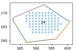
For example, for the cell 24, which is 14 in index, we can have:

All Vertices:

Index = 14
[Vertic for Vertic in vor.ridge_vertices if Vertic[0] in
 vor.regions[vor.point_region[Index]] and Vertic[1] in
 vor.regions[vor.point_region[Index]]]

[[18, 19], [15, 18], [24, 25], [6, 25], [6, 19], [15, 24]]

Index = 0
fig, ax = plt.subplots(figsize = ((df.row.max() - df.row.min())/28, (df.col.max() - df.col.min())/28))

sns.scatterplot(data=df, x= "row", y="col", hue = "r", linewidth = 0, palette= "Paired", legend = None )

for index in range(len(Label_TB)):
  plt.text(x= Label_TB.row.iloc[index],
  y=Label_TB.col.iloc[index],
  s= str(int(Label_TB.r.iloc[index])),
  horizontalalignment='center',
  verticalalignment='center',
)

for Re in vor.regions[vor.point_region[Index]]:
  [sns.lineplot(x=vor.vertices[line][:,0], y = vor.vertices[line][:,1]) for line in vor.ridge_vertices if -1 not in line and Re in line]
sns.lineplot([1,1],[1,1]).set(xlim=(df.row.min(),df.row.max()), ylim=(df.col.min(),df.col.max()))
plt.show()

More precisely, we can have the vertices for a single polygon:

sns.scatterplot(data=df[df.r==24], x= "row", y="col", hue = "r", linewidth = 0, palette= "Paired", legend = None )

plt.text(x= Label_TB.row.iloc[Index],
  y=Label_TB.col.iloc[Index],
  s= str(int(Label_TB.r.iloc[Index])),
  horizontalalignment='center',
  verticalalignment='center',
)


for line in [Vertic for Vertic in vor.ridge_vertices if Vertic[0] in
 vor.regions[vor.point_region[Index]] and Vertic[1] in
 vor.regions[vor.point_region[Index]]]:
  sns.lineplot(x=vor.vertices[line][:,0], y = vor.vertices[line][:,1])

plt.show()

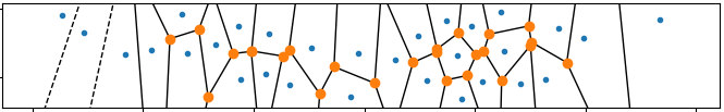
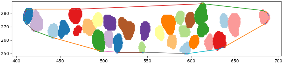
Resolution for cont adjacent cells

1. calculate the points for the boundary
2. Add the boundary points to the group and calculate the Voronoi Spacial
3. Calculate adjacent points by Delaunay
4. Correct Adjacent points by shared boundary

Boundary points

Codes

define the function

def alpha_shape(points, alpha, only_outer=True):
    """
    Compute the alpha shape (concave hull) of a set of points.
    :param points: np.array of shape (n,2) points.
    :param alpha: alpha value.
    :param only_outer: boolean value to specify if we keep only the outer border
    or also inner edges.
    :return: set of (i,j) pairs representing edges of the alpha-shape. (i,j) are
    the indices in the points array.
    """
    assert points.shape[0] > 3, "Need at least four points"
    def add_edge(edges, i, j):
        """
        Add an edge between the i-th and j-th points,
        if not in the list already
        """
        if (i, j) in edges or (j, i) in edges:
            # already added
            assert (j, i) in edges, "Can't go twice over same directed edge right?"
            if only_outer:
                # if both neighboring triangles are in shape, it's not a boundary edge
                edges.remove((j, i))
            return
        edges.add((i, j))
    tri = Delaunay(points)
    edges = set()
    # Loop over triangles:
    # ia, ib, ic = indices of corner points of the triangle
    for ia, ib, ic in tri.vertices:
        pa = points[ia]
        pb = points[ib]
        pc = points[ic]
        # Computing radius of triangle circumcircle
        # www.mathalino.com/reviewer/derivation-of-formulas/derivation-of-formula-for-radius-of-circumcircle
        a = np.sqrt((pa[0] - pb[0]) ** 2 + (pa[1] - pb[1]) ** 2)
        b = np.sqrt((pb[0] - pc[0]) ** 2 + (pb[1] - pc[1]) ** 2)
        c = np.sqrt((pc[0] - pa[0]) ** 2 + (pc[1] - pa[1]) ** 2)
        s = (a + b + c) / 2.0
        area = np.sqrt(s * (s - a) * (s - b) * (s - c))
        circum_r = a * b * c / (4.0 * area)
        if circum_r < alpha:
            add_edge(edges, ia, ib)
            add_edge(edges, ib, ic)
            add_edge(edges, ic, ia)
    return edges

Calculate the index of edge-points

Points = df[['row', 'col']].to_numpy()
edges = alpha_shape(Points, alpha=500, only_outer=True)

fig, ax = plt.subplots(figsize = ((df.row.max() - df.row.min())/28, (df.col.max() - df.col.min())/28))

sns.scatterplot(data=df, x= "row", y="col", hue = "r", linewidth = 0, palette= "Paired", legend = None ).invert_yaxis()

for i, j in edges:
    plt.plot(Points[[i, j], 0], Points[[i, j], 1], color="white")

plt.show()

Calculate Voronoi space with edge-points

# Collect edge-points
Edges = np.array([[i[0], i[1]]for i in edges]).ravel()
Edges = np.unique(Edges)

Edge_points = np.array([Points[i] for i in Edges])

points = Label_TB[['row', 'col']].to_numpy()

Vo_Point = (np.concatenate([points, Edge_points]))


vor = Voronoi(Vo_Point)
voronoi_plot_2d(vor)

fig, ax = plt.subplots(figsize = ((df.row.max() - df.row.min())/28, (df.col.max() - df.col.min())/28))

sns.scatterplot(data=df, x= "row", y="col", hue = "r", linewidth = 0, palette= "Paired", legend = None )

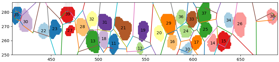
for index in range(len(Label_TB)):
  plt.text(x= Label_TB.row.iloc[index],
  y=Label_TB.col.iloc[index],
  s= str(int(Label_TB.r.iloc[index])),
  horizontalalignment='center',
  verticalalignment='center',
)

#plt.imshow(NP_result.all()['img'])
[sns.lineplot(x=vor.vertices[line][:,0], y = vor.vertices[line][:,1]) for line in vor.ridge_vertices if -1 not in line]
sns.lineplot([1,1],[1,1]).set(xlim=(df.row.min(),df.row.max()), ylim=(df.col.min(),df.col.max()))
plt.show()

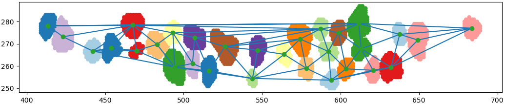
Delaunay to determine near points

from scipy.spatial import Delaunay
from collections import defaultdict
import itertools

tri = Delaunay(points)
neiList=defaultdict(set)
for p in tri.vertices:
    for i,j in itertools.combinations(p,2):
        neiList[i].add(j)
        neiList[j].add(i)

fig, ax = plt.subplots(figsize = ((df.row.max() - df.row.min())/28, (df.col.max() - df.col.min())/28))
plt.triplot(points[:,0], points[:,1], tri.simplices, color="black")
plt.plot(points[:,0], points[:,1], 'o')

sns.scatterplot(data=df, x= "row", y="col", hue = "r", linewidth = 0, palette= "Paired", legend = None )

for index in range(len(Label_TB)):
  plt.text(x= Label_TB.row.iloc[index],
  y=Label_TB.col.iloc[index],
  s= str(int(Label_TB.r.iloc[index])),
  horizontalalignment='center',
  verticalalignment='center',
)

[sns.lineplot(x=vor.vertices[line][:,0], y = vor.vertices[line][:,1]) for line in vor.ridge_vertices if -1 not in line]
sns.lineplot([1,1],[1,1]).set(xlim=(df.row.min(),df.row.max()), ylim=(df.col.min(),df.col.max()))
plt.show()

Correct Adjacent points by shared boundary

def Get_vertices(Index, vor):
  return [Vertic for Vertic in vor.ridge_vertices if Vertic[0] in
 vor.regions[vor.point_region[Index]] and Vertic[1] in
 vor.regions[vor.point_region[Index]]]


Adjacent_dic = {}

for Source in neiList.keys():
  Source_Vtc = Get_vertices(Source, vor)
  for Target in neiList[Source]:
    Tar_Vtc = Get_vertices(Target, vor)
    Result = [i for i in Tar_Vtc if i in Source_Vtc]
    if len(Result)!= 0 :
      print(Source+10, Target+10)

Adjacent_dic = {}

for Source in neiList.keys():
  Source_Vtc = Get_vertices(Source, vor)
  for Target in neiList[Source]:
    Tar_Vtc = Get_vertices(Target, vor)
    Result = [i for i in Tar_Vtc if i in Source_Vtc]
    if len(Result)!= 0 :
      print(Source+1, Target+1)
      if Source + 1 not in Adjacent_dic.keys():
        Adjacent_dic.update({Source+1: [Target+1]})
      else:
        Adjacent_dic[Source+1] += [Target+1]

Ellipse Regression (Fit)

import cv2
import numpy as np
from matplotlib.patches import Ellipse

img = cv2.imread('mask.png', 0)

img[img>=63.22401581839193] = 255
img[img<=24.62768758842168,] = 255
TMP = pd.DataFrame(img)
TMP['Y'] = TMP.index
TMP_L = TMP.melt(id_vars='Y')
TMP_L = TMP_L[TMP_L.value!= 255]

# Convert data to the correct format
X = np.array([[i, ii] for i,ii in zip(x_points, y_points)])

# Fit ellipse
ellipse = cv2.fitEllipse(TMP_L[['Y', "variable"]].to_numpy().astype(int))

fig, ax = plt.subplots()
ax.scatter(TMP_L.Y, TMP_L.variable)
#ax.set_aspect("equal")
ellipse_patch = Ellipse(ellipse[0], width=ellipse[1][0], height=ellipse[1][1], angle=ellipse[2], facecolor='red', alpha=0.5)
ax.add_artist(ellipse_patch)
plt.show()

center: ellipse[0]
major axis: ellipse[1][1]
minor axis: ellipse[1][0]
angle: ellipse[2]

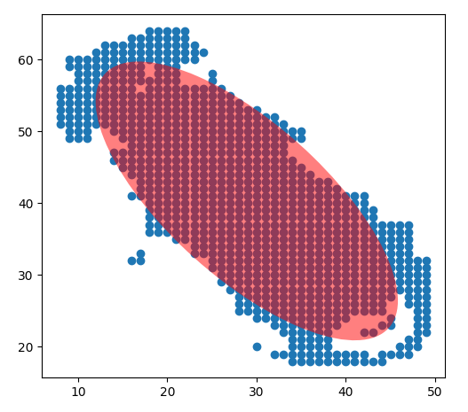
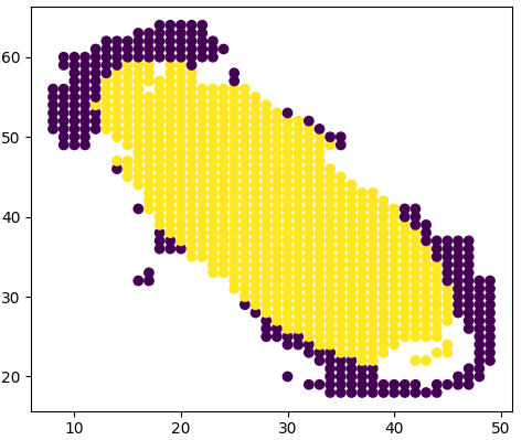
Calculate the point if it is in the ellipse

from numpy.linalg import eig, inv

def point_in_ellipse(point, center, width, height, angle):
    # Convert the point and center to the ellipse-centered coordinate system
    cos_a = np.cos(angle)
    sin_a = np.sin(angle)
    x, y = point[0] - center[0], point[1] - center[1]
    x_ = cos_a*x + sin_a*y
    y_ = -sin_a*x + cos_a*y
    cx, cy = 0, 0

    # Calculate the semi-major and semi-minor axes of the transformed ellipse
    a_ = width/2
    b_ = height/2

    # Check if the transformed point is inside the unit circle
    if ((x_ - cx)/a_)**2 + ((y_ - cy)/b_)**2 <= 1:
        return True
    else:
        return False


# TMP_L is from the code above
TMP_L['Color'] = [point_in_ellipse(TMP_L[['Y', 'variable']].iloc[i], ellipse[0], ellipse[1][0], ellipse[1][1], np.radians(ellipse[2])) for i in range(len(TMP_L))]

plt.scatter(TMP_L.Y, TMP_L.variable, c = TMP_L.Color)
plt.show()