library(ggbio)
library(stringr)
library(reshape2)
library(Rsamtools)
library(rtracklayer)
library(org.Dm.eg.db)
library(GenomicFeatures)
library(clusterProfiler)
library(VariantAnnotation)
library(BSgenome.dme.BDGP6.32)
GTF= "/media/ken/BackUP/Drosophila/Drosophila_melanogaster.BDGP6.32.104.chr.EGFP.GAL4.mCD8GFP.gtf"
txdb <- makeTxDbFromGFF(file=GTF, format="gtf")
Trans <- transcriptsBy(txdb, "gene")
tmp <- bitr(names(Trans), fromType="FLYBASE", toType="SYMBOL", OrgDb="org.Dm.eg.db")
names(Trans)[!is.na(tmp[[2]][match(names(Trans), tmp[[1]])])] <- tmp[[2]][match(names(Trans), tmp[[1]])][!is.na(tmp[[2]][match(names
(Trans), tmp[[1]])])]
BAM_Dir = "/run/user/1000/gvfs/sftp:host=cypress1.tulane.edu,user=wliu15/lustre/project/wdeng7/wliu15/Bam/"
VCF_Dir = "/run/user/1000/gvfs/sftp:host=cypress1.tulane.edu,user=wliu15/lustre/project/wdeng7/wliu15/vcf/"
Bam_list <- c("wt_10day_1_S27Aligned.sortedByCoord.out.bam",
"G1F1_S31Aligned.sortedByCoord.out.bam",
"G50-FE_TUMOR-a_S37Aligned.sortedByCoord.out.bam"
)
GENE = "N"
RNA_plot <- function(GENE){
tmp = range(Trans[GENE])[[1]]
wh = as(c(paste(tmp@seqnames@values, ":", tmp@ranges@start, "-", tmp@ranges@start+tmp@ranges@width, sep ="")), "GRanges")
rg = c(tmp@ranges@start, tmp@ranges@start+tmp@ranges@width)
Result = c()
Result2 = c()
for (sample in Bam_list){
VCF <- read.table(paste(VCF_Dir, sample, ".vcf", sep=''))
bam<-BamFile(file=paste(BAM_Dir, sample, sep=""), index=paste(BAM_Dir, sample, ".bai", sep=""))
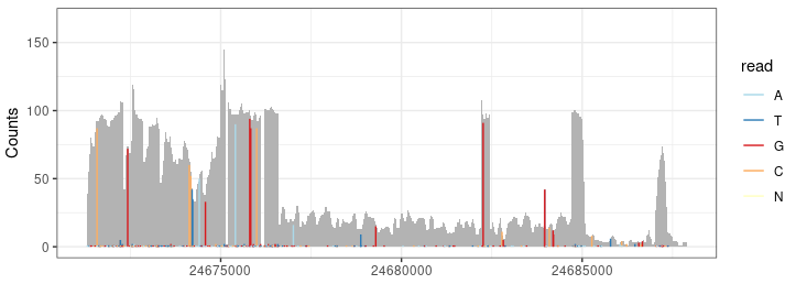
P2 <- autoplot(bam, which =wh, bsgenome =BSgenome.dme.BDGP6.32, stat = "mismatch") + theme_bw() + guides(color=guide_legend(title=""))
Result <- c(Result, P2)
TB <- VCF[VCF$V1== as.character(tmp@seqnames@values),]
TB <- TB[TB$V2>=min(rg),]
TB <- TB[TB$V2<=max(rg),]
TB <- TB[c("V2", "V4", "V5")]
colnames(TB) <- c("x", "Ref", "Alt")
TB <- melt(TB, id.vars = "x" )
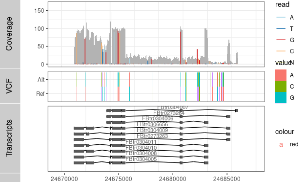
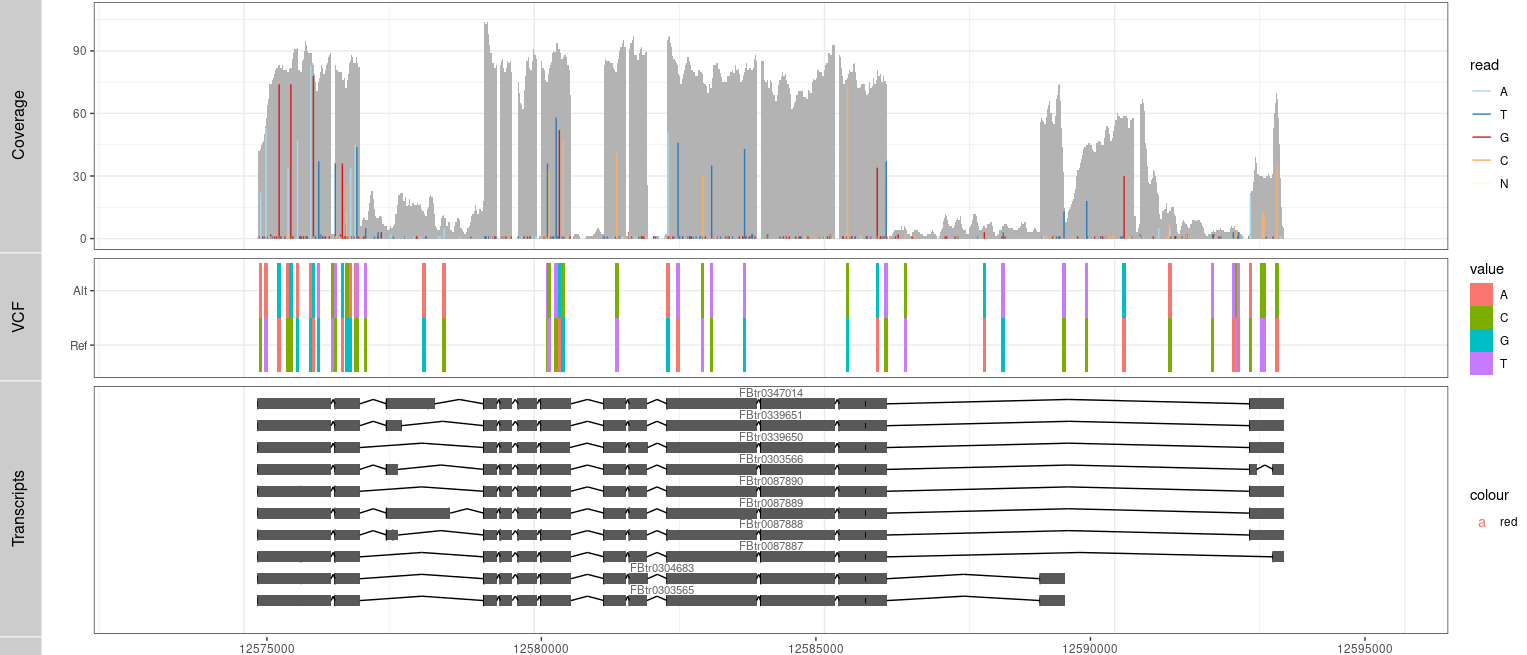
P3 <- ggplot() + geom_tile(data=TB,aes(x= x, y= variable, label=value, fill= value), width=(rg[2]-rg[1])/300) +
coord_cartesian(xlim =rg, expand = T) + theme_bw()
Result2 <- c(Result2, P3)
}
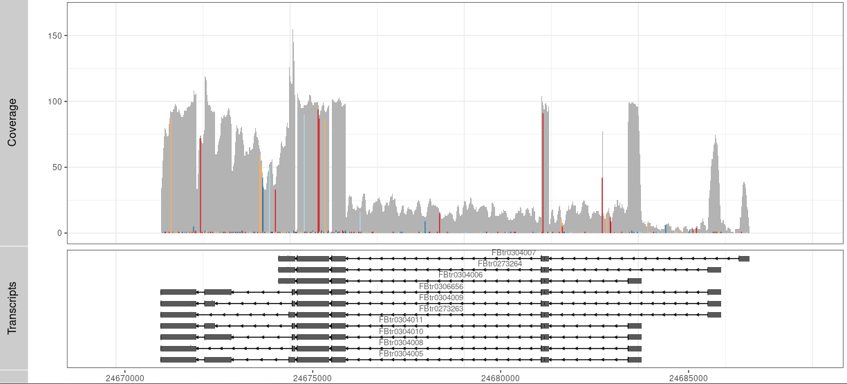
P1 <- autoplot(txdb, which= wh)+ theme_bw() +
geom_text(aes(x=0, y=0, label=0,color="red"))+
coord_cartesian(xlim =rg, expand = T)
tracks( c(Result,P1))
ggsave(paste("img/", GENE, '_RNA.png',sep= ""), w= 20 , h= 5.45)
}
ggsave("~/tmp/Mutation_GTF.png", w= 20 , h= 1.55)
|