Unmapped reads Annotations

Why Unmapped Reads

Though we expect that the microbes are free in normal/healthy animal tissue, organ, or brain, we still get a few unmapped reads from NGS. And most of them are contributed by microbes. A Gouin, et al., 2014[1] studied those unmapped reads from 33 plants and believed that those sequences may contribute to the divergence between host plant specialized biotypes.

To identify those unmapped reads, lots of pipelines and tools are developed. Mara Sangiovanni, 2019[2] published the DecontaMiner for investigating the presence of contamination. Zifan Zhu, 2019[3] released MicroPro to study the know and unknown microbes based on the unmapped reads.

Not only in DNA-seq, but RNA-seq could also find lots of unmapped reads and they could be meaningful, too. Artur Gurgul, et al., 2022 [4] found those unmapped reads not only comes from contamination but also come from the hosts and could be used to refine the reference genome. For example, Majid Kazemian, 2015[5] find lots of new or abnormal transcripts from human cancer RNA-seq. A few de novo contigs from unmapped reads could not align to humans but other few kinds of Primates have positive effects on the tumor cell.

Possible sources of unmapped reads:

  • Biology Issue
    • Human (From the technician)
    • symbionts/pathogens
      • Viruses
      • Bacteria
      • fungi
      • other parasites (exp, mites)
    • repetitive elements (some alignment tools would ignore them)[4:1]
    • genetic variation
      • SCGB1A1 gene(RNA-seq) [4:2]
      • absent or misassembled in the reference genome[6]
    • Not well-identified Genes[4:3]
    • non-coding RNA (RNA-seq)[4:4]
  • Technical Issue
    • primer-dimer formation[7]
    • Cloning/Expression Vecters

Once we realized the existence and significance of unmapped reads, we need to find a way to annotate and analyze them. Kraken2 and bracken could be good choose.

Published Pipeline

A Gouin, 2014[1:1]:

Host: 33 pea aphid
Host Genome; mitochondrial genome; primary bacterial symbiont; several secondary symbiont genomes reported for the pea aphid.

Main Steps Software Function
Find unmapped reads Bowtie2 align to Reference Genome
Find unmapped reads Samtools extract unmaped reads
Unmapped reads assembly Prinseq trimme the quality below 20 within a window of 10 nucleotides, and only sequences of at least 66 nucleotides in length were retained
Unmapped reads Analysis Compareads Find similar reads between two sets of reads in an assembly-free manner
Unmapped reads assembly ABySS Unmapped reads de novo assembling
Unmapped reads assembly Bowtie2 align unmapped reads to assembled Contigs
Contigs analysis BLASTClust Found homologous large contigous.
Contigs analysis BLASTn Found homologous contigous
Unmapped reads assembly readFilter only reads for which 68% of the length was covered by 31-mers present at least 100 times in the data set were retained
Unmapped reads assembly SPAdes De novo assembly
Potentially divergent Mummer Global aligner, against reference: >80% identity and >500 bp were retained
Contigs analysis GeneMarkS+ Predict the protein from de novo contigs.
Contigs analysis Blastp Predicted protein annotation
Potentially divergent Stampy An aligner performs well when divergent is high.
Potentially divergent GATK SNP calling

PS:

  • Why Bowtie2: the percentage of unmapped reads was higher than for Bowtie2 (on average over the 33 individuals, 6.1% vs 3.7% for BWA and Bowtie2, respectively)

DecontaMiner, 2019[2:1]

© Mara Sangiovanni, et al. 2019

MicroPro, 2019[3:1]

    1. Align reads to Reference-based known microbial by Centrifuge
    • The average mapping rate for each dataset is about 35–40%.
    1. Cross-assembly by: Megahit and Minia 3
    • Megahit performed better in real data analysis.
    • MetaBAT 2.12.1 to binning
    • Abundance estimate achived by BWA-aln
    1. Predicting phenotypes using random forests

About viral:

  • Step 1: Known viral abundance extraction
  • Step 2: Unknown viral feature detection
  • Step 3: Predicting phenotypes based on viral abundance

PS: Corss-assembly:

Using reads from different samples to assemble: Increasing the coverage of contigs.B. Papudeshi; 2018

Unmapped human RNA-Seq data and their association with cancer

© Majid Kazemian, 2015

Exploring the unmapped DNA and RNA reads in a songbird genome

© Veronika N. Laine, 2015

About Bracken

  • Jen Lu; 2017: If a 150bp read is 100% identical to two different species, Kraken will assign it to their lowest common ancestor (LCA), which could be at the genus level or higher. But some reads within a particular sample usually come from the unique (or species-specific) portion of the genome. Bracken uses this information, plus information about the similarity between the sister species, to “push down” reads from the genus level to the species level.
  • Other background information: Challenges in benchmarking metagenomic profilers; Nature Methods

To be notices, Kraken2 and Bracken is DNA-to-DNA strategy. The abundance of the reads is relative to the nucleotide, not species individual.

© Zheng Sun, 2021

Why Kraken

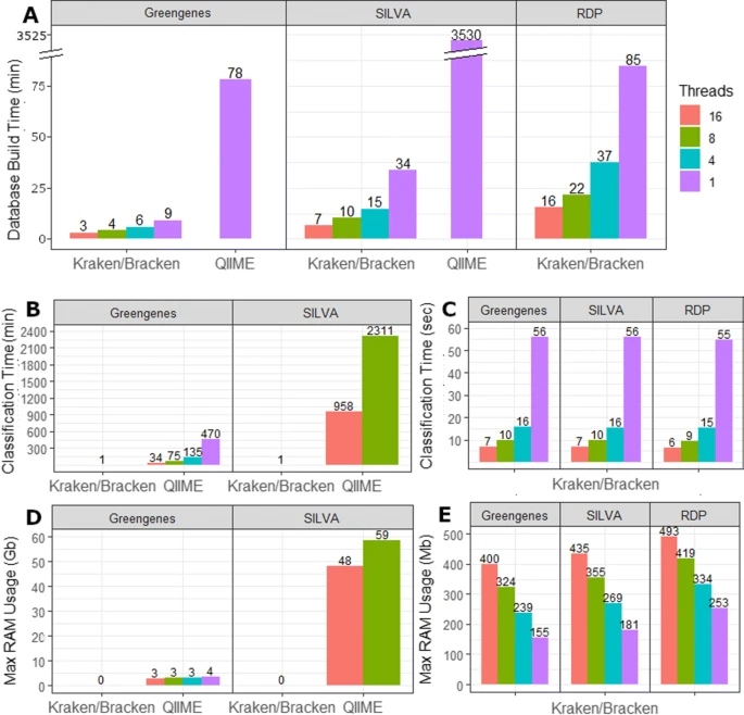
Lu J., et al. showed that comparing to QiiMe, Kraken2 has uncompetable speed in annotation and the results from kraken-bracken are even better than QiiMe[8]. I think it’s time for QiiMe move a room for Kraken2 now.

© Lu J.

Unmapped reads

Prepare your working directories

.
├── Bam
├── FQ_unmapped
├── Parasites
├── Log
├── Model.sh
└── script
  • Bam: Aligned bam files
  • FQ_unmapped: Storing the unmapped reads from .bam
  • Parasites: Directory for store Clean.fa which contains some contamination seqs and cloning vectors.
  • Log: Directory for logs
  • Model.sh: A script with slurm parameters.
  • script: script for

A Quick Pipeline from Genomics Tutorial; 2020:

Prepare Database

Prepare your vector sequence in `vector.fa`

mkdir Parasites
cd Parasites
wget https://ftp.ncbi.nlm.nih.gov/genomes/all/GCF/000/010/205/GCF_000010205.1_ASM1020v1/GCF_000010205.1_ASM1020v1_genomic.fna.gz
wget https://ftp.ncbi.nlm.nih.gov/genomes/all/GCF/000/239/435/GCF_000239435.1_ASM23943v1/GCF_000239435.1_ASM23943v1_genomic.fna.gz
wget https://ftp.ncbi.nlm.nih.gov/genomes/all/GCF/000/255/335/GCF_000255335.2_Mocc_1.1/GCF_000255335.2_Mocc_1.1_genomic.fna.gz

curl -OJX GET "https://api.ncbi.nlm.nih.gov/datasets/v1/genome/accession/GCA_024678965.1/download?include_annotation_type=GENOME_GFF,RNA_FASTA,CDS_FASTA,PROT_FASTA&filename=GCA_024678965.1.zip" -H "Accept: application/zip"

gunzip *
sed "s/>/>Mite_/" *.fna > Clean.fa
unzip GCA_024678965.1.zip
sed "s/>/>nematodes_/" ncbi_dataset/data/GCA_024678965.1/GCA_024678965.1_AAFC-BrLi-01_v2_genomic.fna >> Clean.fa
cat vector.fa >> Clean.fa

Unmapped reads extraction

  • Align to Reference Genome → Unmapped reads extract → Kraken2 annotation → Bracken Abundance estimation.

Technically, you can find the unmapped reads by samtools view *.bam| awk '$3=="*"'. But I don’t know why the number of reads is less than the result from samtools stats. So, the easiest way to achieve this is:

  • Single end: samtools fastq -@ 8 -f 4 Bam/S10_aln_pe_bqsr.bam > s.fq.gz
  • Paired end:
    samtools fastq -@ 8 -f 4 Bam/10_aln_pe_bqsr.bam -1 1.fq.gz -2 2.fq.gz -s s.fq.gz

In this code, reads would be split into 3 files: 1.fq.gz, 2.fq.gz, and s.fq.gz. The first two are paired reads and the 3rd is unpaired reads. In Kraken classification under paired parameter, unpaired reads in fq file would be ignored. So, we need to store them independently and run kraken twice.

If some samples are single ends, the result cannot be stored with this command. But the reads would be printed into log file: Log/*.out. So, we can compress it into fq.gz

module load samtools

SUFFIX=_aln_pe_bqsr.bam
BAM=Bam
OUT_dir=FQ_unmapped

mkdir $OUT_dir script Log
for i in $(ls $BAM/*.bam);
do SAMPLE=$(echo $i| awk -F"/" '{print $NF}'| sed "s/$SUFFIX//");
if [ -f $OUT_dir/$SAMPLE\_1.fq.gz ];
then echo $SAMPLE is done
else
sed "s/Hi/$SAMPLE/" Model.sh > script/$SAMPLE\_fq.sh
echo "samtools fastq -@ 8 -f 4 $i -1 $OUT_dir/$SAMPLE""_1.fq.gz -2 $OUT_dir/$SAMPLE""_2.fq.gz -s $OUT_dir/$SAMPLE""_s.fq.gz" >> script/$SAMPLE\_fq.sh
sbatch script/$SAMPLE\_fq.sh
fi
done

# Check for Single Ends

for i in $(du Log/*.out | grep -v ^0|awk '{print $2}');
do SAMPLE=$(echo $i| sed 's=Log/==;s/.out//')
sed "s/Hi/Single_$SAMPLE/" Model.sh > script/$SAMPLE\_fq_s.sh
echo gzip -c $i \> $OUT_dir/$SAMPLE\_s.fq.gz >> script/$SAMPLE\_fq_s.sh
sbatch script/$SAMPLE\_fq_s.sh
done

# Finally, remove emplty fq files
rm $(du $OUT_dir/*| grep "^4"$'\t'|awk '{print $2}')

# Check the number of samples is correct or not
ls $OUT_dir/*|sed 's/_[12s].fq.gz//'|sort|uniq |wc -l
131

Here I have 131 samples in total. And result is 131 which means I didn’t miss any of them.

If you are not using slurm syste, this code may help

for SAMPLE in $(du FQ_unmapped/_s.fq.gz | grep ^4$'\t'| awk -F"/" '{print $NF}'| sed 's/_s.fq.gz//');
do i=$(ls $BAM/
.bam| grep $SAMPLE)
echo $SAMPLE $i
samtools fastq -@ 8 -f 4 $i > FQ_unmapped/$SAMPLE_s.fq.gz
done

Align into Cleaning database and counts

cd Parasites
bwa index Clean.fa
cd ..

Here we already know that the fq ends as 1_fq.gz is Paired reads, s_fq.gz is unpaired reads. So, we can do:

FQ_DB=FQ_unmapped
DB=Parasites
DB_FA=Parasites/Clean.fa
OUTPUT=Bam_clean

mkdir $OUTPUT

# Paired
for SAMPLE in $(ls $FQ_DB/*_1.fq.gz| sed "s=$FQ_DB/==;s/_[12].fq.gz//"); do
if [ -f $SAMPLE.P.sorted.bam ]; then
echo $SAMPLE is done
else
echo $SAMPLE can not be find
sed "s/Hi/$SAMPLE\_P_$DB/" Model.sh > script/$SAMPLE\_P_$DB.sh
echo bwa mem $DB_FA $FQ_DB/$SAMPLE\_1.fq.gz $FQ_DB/$SAMPLE\_1.fq.gz -t 64 \|samtools view -S -b -\|samtools sort \> $SAMPLE.P.sorted.bam >> script/$SAMPLE\_P_$DB.sh
echo samtools index $SAMPLE.P.sorted.bam >> script/$SAMPLE\_P_$DB.sh
sbatch script/$SAMPLE\_P_$DB.sh
fi
done

# Single
for SAMPLE in $(ls $FQ_DB/*_s.fq.gz| sed "s=$FQ_DB/==;s/_s.fq.gz//"); do
if [ -f $SAMPLE.S.sorted.bam ]; then
echo $SAMPLE is done
else
echo $SAMPLE can not be find
Clean
echo bwa mem $DB_FA $FQ_DB/$SAMPLE\_s.fq.gz -t 64 \|samtools view -S -b -\|samtools sort \> $SAMPLE.S.sorted.bam >> script/$SAMPLE\_S_$DB.sh
echo samtools index $SAMPLE.S.sorted.bam >> script/$SAMPLE\_S_$DB.sh
sbatch script/$SAMPLE\_S_$DB.sh
fi
done

## Check unexpected size of file
rm $(du *.sorted.bam | awk '$1<=100'| awk '{print $2}')
## After removed failed files, we can excute the for loop again
#.
#.
#.
## finally, we can mv all bam into another directory
mv *.sorted.* $OUTPUT

Counting results

There are two bam files. One is paired result, another is single end result. For avoid counting them twice in paired result, we can samply sort and uniq them. The only problem is it would consume lots of memory and time.

for SAMPLE in $(ls Bam_clean/*.bam| sed 's/.[PS].sorted.bam//;s=Bam_clean/=='| sort |uniq);
do sed "s/Hi/$SAMPLE_Clean_count/" Model.sh > script/$SAMPLE.bam_count.sh
echo "cat Bam_clean/$SAMPLE.[PS].sorted.bam| samtools view| awk '{print $1,$3}'| awk -F"_" '{print $1}'| sort|uniq| awk '{print $2}'|sort| uniq -c |sed 's/^ *//'> Bam_Stats/$SAMPLE.Clean.csv" >> script/$SAMPLE.bam_count.sh
sbatch script/$SAMPLE.bam_count.sh
done

extract unmapped reads again

Codes folded for extract reads again
module load samtools

BAM=Bam_clean
OUT_dir=FQ_split

mkdir $OUT_dir script Log

## paired-end reads
for i in $(ls $BAM/*.P.sorted.bam);
do SAMPLE=$(echo $i| awk -F"/" '{print $NF}'| sed "s/.P.sorted.bam//");
if [ -f $OUT_dir/$SAMPLE\_1.fq.gz ];
then echo $SAMPLE is done
else
sed "s/Hi/$SAMPLE/" Model.sh > script/$SAMPLE\_fq.sh
echo "samtools fastq -@ 8 -f 4 $i -1 $OUT_dir/$SAMPLE""_1.fq.gz -2 $OUT_dir/$SAMPLE""_2.fq.gz -s $OUT_dir/$SAMPLE""_s.fq.gz" >> script/$SAMPLE\_fq.sh
sbatch script/$SAMPLE\_fq.sh
fi
done

# Check for Single Ends

for i in $(ls $BAM/*.S.sorted.bam);
do SAMPLE=$(echo $i| awk -F"/" '{print $NF}'| sed "s/.S.sorted.bam//");
sed "s/Hi/$SAMPLE/" Model.sh > script/$SAMPLE\_fq.sh
echo "samtools fastq -@ 8 -f 4 $i| gzip -f > $OUT_dir/$SAMPLE""_s.fq.gz" >> script/$SAMPLE\_fq.sh
sbatch script/$SAMPLE\_fq.sh
done

# Finally, remove emplty fq files
rm $(du $OUT_dir/*| grep "^4"$'\t'|awk '{print $2}')

# Check the number of samples is correct or not
ls $OUT_dir/*|sed 's/_[12s].fq.gz//'|sort|uniq |wc -l

A Quick Pipeline Example

  1. Create a virtual environment and install tools
  2. Prepare the test data (fastq)
  3. Prepare the database (virus Kraken database)
  4. Run the result
  5. Bracken correction

More annotation database could be found: GitHub Kraken2 DataBase

# 1. Creat a virtual environment
conda create --yes -n kraken -c bioconda kraken2 bracken
conda activate kraken

# 2. Download Test data
wget -O mappings.tar.gz https://osf.io/g5at8/download
tar xvzf mappings.tar.gz

mkdir kraken
cd kraken

# 3. download annotation database
mkdir Viral
cd Viral
wget https://genome-idx.s3.amazonaws.com/kraken/k2_viral_20220607.tar.gz
tar -zxvf k2_viral_20220607.tar.gz
cd ..

# 4. Run the resutls
DB=Viral

# 5. Branken correction
kraken2 --use-names --threads 4 --db PlusPFP --fastq-input --report $DB.report --gzip-compressed --paired ../mappings/evol1.sorted.unmapped.R1.fastq.gz ../mappings/evol1.sorted.unmapped.R2.fastq.gz > $DB.kraken

bracken -d $DB -i $DB.report -o $DB.bracken -r 300 -l S -t 2

Pipeline for Paired reads

mkdir Kraken_result FQ_split

FQ=FQ_split
DB=PlusPFP
DB_L=../kraken/PlusPFP
# paired
for SAMPLE in $(ls $FQ/*_1.fq.gz| sed "s/_1.fq.gz//;s=$FQ/=="); do
if [ -f Kraken_result/$SAMPLE\_$DB\_P.bracken ];then
echo $SAMPLE is done
else
echo Try $SAMPLE
sed "s/Hi/Kra_$SAMPLE/" Model.sh > script/kraken_$SAMPLE\_P.sh
echo kraken2 --use-names --threads 64 --db $DB_L --fastq-input --report Kraken_result/$SAMPLE\_$DB\_P.report --gzip-compressed --paired $FQ/$SAMPLE\_1.fq.gz $FQ/$SAMPLE\_2.fq.gz \> Kraken_result/$SAMPLE\_$DB\_P.kraken >> script/kraken_$SAMPLE\_P.sh
echo bracken -d $DB_L -i Kraken_result/$SAMPLE\_$DB\_P.report -o Kraken_result/$SAMPLE\_$DB\_P.bracken -r 300 -l S -t 2 >> script/kraken_$SAMPLE\_P.sh
sbatch script/kraken_$SAMPLE\_P.sh
fi
done

# sangle
for SAMPLE in $(ls $FQ/*_s.fq.gz| sed "s/_s.fq.gz//;s=$FQ/=="); do
if [ -f Kraken_result/$SAMPLE\_$DB\_S.bracken ];then
echo $SAMPLE is done
else
echo Try $SAMPLE
sed "s/Hi/Kra_$SAMPLE/" Model.sh > script/kraken_$SAMPLE\_S.sh
echo kraken2 --use-names --threads 64 --db $DB_L --fastq-input --report Kraken_result/$SAMPLE\_$DB\_S.report --gzip-compressed --paired $FQ/$SAMPLE\_s.fq.gz $FQ/$SAMPLE\_s.fq.gz \> Kraken_result/$SAMPLE\_$DB\_S.kraken >> script/kraken_$SAMPLE\_S.sh
echo bracken -d $DB_L -i Kraken_result/$SAMPLE\_$DB\_S.report -o Kraken_result/$SAMPLE\_$DB\_S.bracken -r 300 -l S -t 2 >> script/kraken_$SAMPLE\_S.sh
sbatch script/kraken_$SAMPLE\_S.sh
fi
done

For other levels:
Levels: D → K → P → C → O → F → G → S
EXP:

D	Eukaryota
K	  Metazoa
P	   Chordata
C	    Mammalia
O	     Primates
F	      Hominidae
G	       Homo
S	        Homo sapiens
DB=PlusPFP
LEVEL=G
for SAMPLE in $(ls FQ_split/*.fq.gz| sed 's/_[12].fq.gz//;s=FQ_split/=='|sort |uniq); do
bracken -d $DB -i Kraken_result/$SAMPLE\_$DB.report -o Kraken_result/$SAMPLE\_$DB\_$LEVEL.bracken -r 300 -l $LEVEL -t 2
done

Combine them into one csv:

grep . Kraken_result/*.bracken| head -n 1| sed 's/:/\t/;s=Kraken_result/==;s/_PlusPFP.bracken//' > bracken.csv
grep -v "taxonomy_id" Kraken_result/*.bracken| sed 's/:/\t/;s=Kraken_result/==;s/_PlusPFP.bracken//' >> bracken.csv

grep "sequences unclassified" Log/Kra_*.err| grep -v nan| awk '{print $1,$2,$NF}'| sed 's/[:/()%]//g;s/LogKra_//;s/.err//' > Unclassed.csv

Extract unclassified reads

# record unclassified reads
for i in $(ls Kraken_result/*.kraken);
do OUT=$(echo $i| sed 's=Kraken_result/==;s/.kraken/.uc.list/')
grep ^U $i| awk '{print $2}' > Log/$OUT
done

RED_dir=FQ_split
OUT_dir=FQ_split2
mkdir $OUT_dir
mkdir $OUT_dir/$RED_dir

# extract unclassified reads with seqkit
for i in $(ls Log/*.uc.list)
do echo $i;
if [ $(echo $i| sed 's/_S.uc.list//') != $i ] ; then
sed "s/Hi/seqkit_S_$SAMPLE/" Model.sh > script/$SAMPLE\_S.sh
READ_1=$(echo $i | sed "s=Log=$RED_dir=;s/_PlusPFP_P.uc.list/_s.fq.gz/")
seqkit grep -n -f $i $READ_1 > $OUT_dir/$READ_1
else
sed "s/Hi/seqkit_S_$SAMPLE/" Model.sh > script/$SAMPLE\_P.sh
READ_1=$(echo $i | sed "s=Log=$RED_dir=;s/_PlusPFP_P.uc.list/_1.fq.gz/")
READ_2=$(echo $i | sed "s=Log=$RED_dir=;s/_PlusPFP_P.uc.list/_2.fq.gz/")
seqkit grep -n -f $i $READ_1 > $OUT_dir/$READ_1
seqkit grep -n -f $i $READ_2 > $OUT_dir/$READ_2
fi
done

Visualization in R

library(ggplot2)
library(ggrepel)

TB <- read.table("Unclassed.csv")
TB$Total <- TB$V2/TB$V3*100

ggplot(TB, aes(x=Total, y= V3)) + geom_point() +
geom_text_repel(aes(label= V1)) + theme_bw() +
coord_cartesian(ylim = c(0,100), expand = F)
Ratio of unclassified Reads

Download SuperKingdom table from NCBI

wget ftp://ftp.ncbi.nih.gov/pub/taxonomy/taxcat.tar.Z
tar -zxvf taxcat.tar.Z

Abbr. Kingdom
A Archaea
B Bacteria
E Eukaryota
V Viruses and Viroids
U Unclassified
O Other (exp. Plasmids)
library(ggplot2)
library(reshape2)
library(stringr)
library(pheatmap)
library(ggrepel)

TB <- read.csv("bracken.csv", sep= '\t', header = T)
Kingdom <- read.table("categories.dmp")

TB$SK <- Kingdom$V1[match(TB$taxonomy_id, Kingdom$V2)]
colnames(TB)[1]="Sample"

SAMPLE = head(unique(TB$Sample), 10)
#SAMPLE = unique(TB$Sample[-grep("[AT][TA]|[Hh][Oo][Ss][tT]|NICD|G17", TB$Sample)])
TMP <- TB[TB$Sample %in% SAMPLE,]
TMP$Sample <- as.factor(as.character(TMP$Sample))
#TMP$Sample <- factor(TMP$Sample, levels = unique(TMP$Sample)[c(1:10,14:18,21,11:13,19:20)])


TB_w <- reshape(TB[c(1,2,8)], timevar = "Sample", idvar = 'name', direction = 'wide')
row.names(TB_w) <- TB_w[[1]]
TB_w <- TB_w[-1]
colnames(TB_w) <- str_replace(colnames(TB_w), "fraction_total_reads.", "")
TB_w[is.na(TB_w)] <- 0


TB_wS <- as.data.frame(t(scale(t(TB_w))))
TB_wS<- TB_wS[!is.na(TB_wS[[1]]),]
pheatmap(TB_wS)

# PCA
TB_wS.pca <- prcomp(t(TB_wS),scale. = F)
TB_wS.pca= data.frame(TB_wS.pca$x)

TB_wS.pca$Group = "Other"
TB_wS.pca$Group[grep("MH",row.names(TB_wS.pca))] <- "MH"
TB_wS.pca$Group[grep("FH",row.names(TB_wS.pca))] <- "FH"

ggplot(TB_wS.pca, aes(PC1,PC2, color=Group)) +
geom_point()+ theme_bw() +
geom_text_repel(aes(label=row.names(TB_wS.pca)))

ggplot(TB_wS.pca[TB_wS.pca$Group %in% c("FH", "MH"),], aes(PC1,PC2, color=Group)) +
geom_point()+ theme_bw() +
geom_text_repel(aes(label=row.names(TB_wS.pca[TB_wS.pca$Group %in% c("FH", "MH"),])))+
stat_ellipse(lwd=1,level = 0.75)

#ggplot(TB, aes(Sample, fraction_total_reads, fill=name)) + geom_bar(stat = 'identity', position = 'fill')
Type Graphics
Pheatmap
PCA

Barplot

ggplot(TB, aes(Sample, new_est_reads, fill=name)) + theme_bw()+
geom_bar(stat = 'identity', position = "fill", show.legend = F)+
theme(axis.text.x = element_text(angle = 90, hjust = 1, vjust = .5))+
facet_grid(SK~.)+ geom_text_repel(aes(label=name), color = "black",
show.legend = F, position = position_fill(vjust= .5))

Relationship with unmapped reads and unclassified reads

.
├── Bam_stats
│   └── SAMPLE.stats.csv
└── Kraken_result
    ├── SAMPLE_PlusPFP.bracken
    ├── SAMPLE_PlusPFP_bracken.report
    ├── SAMPLE_PlusPFP.kraken
    └── SAMPLE_PlusPFP.report

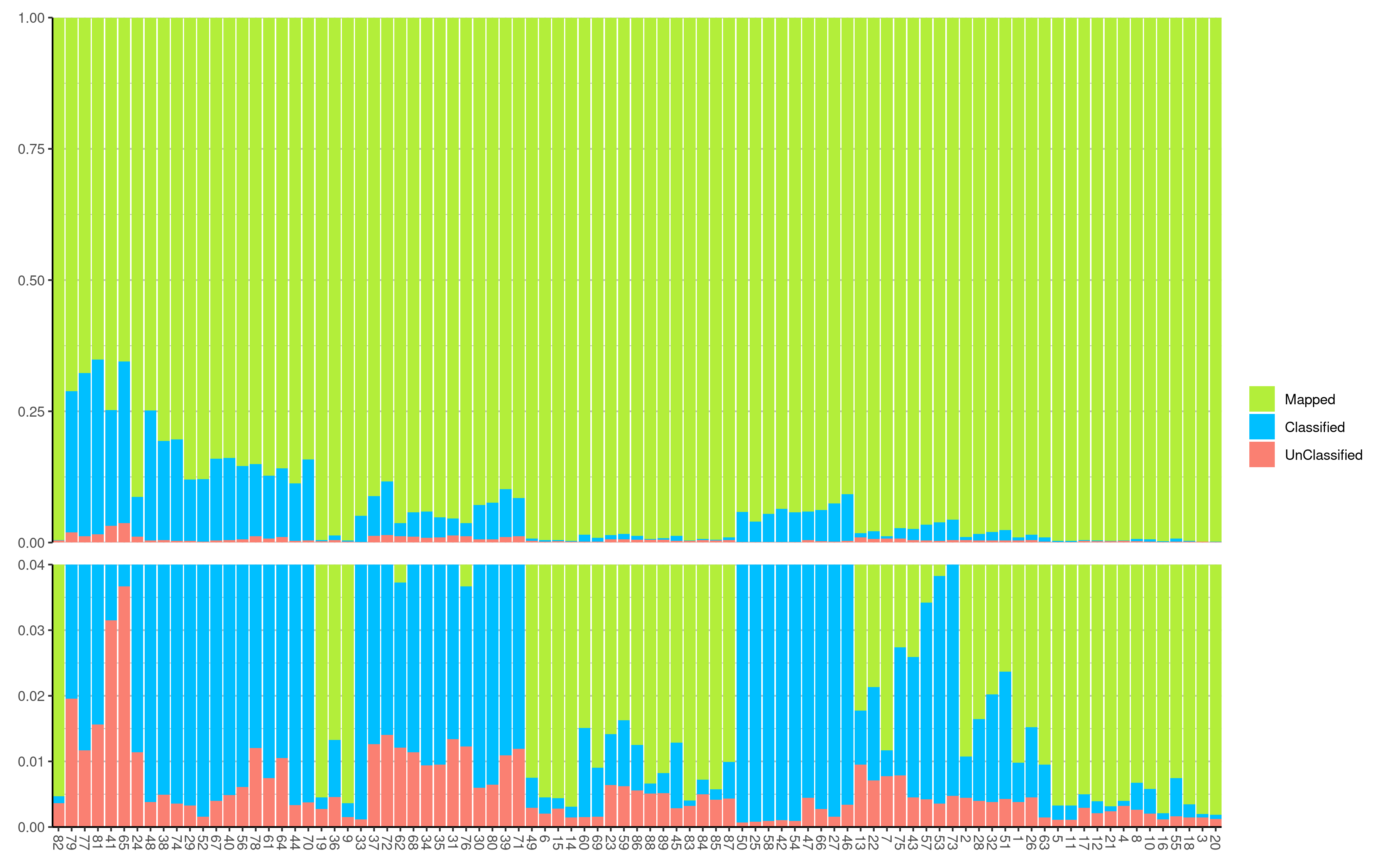
Bams_stats is generated by samtools stats SAMPLE.bam > SAMPLE.stats.csv

In Kraken, when you use paired reads, it would only show the number of the paired reads which means you only get a half size of the reads compared to the result from samtools stats. As a result, we need to multiply them by 2 during visualization.

echo -e "Sample\tTotal\tUnmapped\tClassified\tUnClassified" > Counts_Ratio.csv

for i in $(ls Bam_stats/| sed 's/.stats.csv//');
do
UNMAP=$(grep -w "reads unmapped" Bam_stats/$i.stats.csv| awk -F"\t" '{print $3}')
TOTAL=$(grep -w "raw total sequences:" Bam_stats/$i.stats.csv| awk -F"\t" '{print $3}')
CLASF=$(grep -c ^C Kraken_result/$i\_PlusPFP.kraken)
UNCLF=$(grep -c ^U Kraken_result/$i\_PlusPFP.kraken)
echo -e "$i\t$TOTAL\t$UNMAP\t$CLASF\t$UNCLF"
done >> Counts_Ratio.csv
library(ggplot2)
library(reshape2)
library(pheatmap)
library(ggplotify)
library(ggkaboom)

TB <- read.table("Counts_Ratio.csv", header =T)
#TB$Sample <- as.character(as.numeric(TB$Sample))
TB$Classified <- TB$Classified*2
TB$UnClassified <- TB$UnClassified*2

TB2 <- TB
TB2[3:5] <- TB2[3:5]/TB2[[2]]
TB2[2:5] <- scale(TB2[2:5])
row.names(TB2) <- TB2[[1]]
TB2 <-TB2[-1]
P <- pheatmap(t(TB2))
as.ggplot(P)
ggsave("img/Number_Pheat.png", h= 7.5, w = 12)


# for Bar fill plot
TB_bar <- TB
TB_bar$Mapped <- TB_bar$Total -TB_bar$ Unmapped
TB_bar <- TB_bar[c("Sample", "Mapped", "Classified", "UnClassified")]
#TB_bar_r <- TB_bar[2:4]/TB$Total
#row.names(TB_bar_r) <- TB$Sample

TB.hclust <- hclust(dist(TB2))
TB_L <- melt(TB_bar)
TB_L$Sample <- factor(TB_L$Sample, levels=TB.hclust$labels[TB.hclust$order])
P <- ggplot(TB_L, aes(Sample, value, fill= variable)) +
geom_bar(stat = 'identity', position = 'fill')+theme_bw() +
scale_fill_manual( values= c("OliveDrab2", "deepskyblue", "salmon")) +
theme(axis.text.x = element_text(angle= 270, hjust=0, vjust = .5))

Kaboom_break(P, c(0, 0.04, 0, 1), R=c(2, 1))
ggsave("img/Number_Bar.png", h= 7.5, w = 12)

# Not Fill
TB_bar2 <- melt(TB[c("Sample", "Total", "Unmapped", "UnClassified")])
TB_bar2$Sample <- factor(TB_bar2$Sample, levels=TB.hclust$labels[TB.hclust$order])

P <- ggplot(TB_bar2, aes(Sample, value, fill= variable)) +
geom_bar(stat = 'identity', position = position_identity() )+
scale_fill_brewer(palette = "Set2")+ theme_bw() +
theme(axis.text.x = element_text(angle= 270, hjust=0, vjust = .5))
Kaboom_break(P, c(0, 20000000, 0, 200000000), R=c(2, 1))
ggsave("img/Number_raw.png", h= 7.5, w = 12)

## Unclassified
TB_L$Sample <- factor(TB_L$Sample, levels=TB$Sample[order(TB$UnClassified/TB$Classified)])

P <- ggplot(TB_L[TB_L$variable!="Mapped",], aes(Sample, value, fill= variable)) +
geom_bar(stat = 'identity', position = 'fill')+theme_bw() +
scale_fill_manual( values= c("deepskyblue", "salmon")) +
theme(axis.text.x = element_text(angle= 270, hjust=0, vjust = .5))

ggsave("img/Number_Bar_classR.png", h= 7.5, w = 12)
Header One Header Two

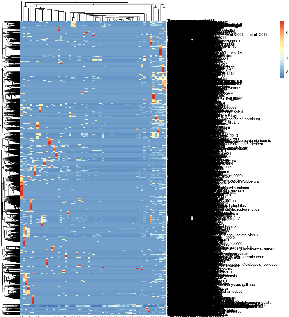
Full Taxonomic information based on ID

Some times, we’d like to analyze the Eucariaotic or Viral independently. Them, we need to find the phlums of them based on taxonomic ID. etetoolkit Can help find the phylums efficiently.

conda create -n ete3 python=3
conda activate ete3
conda install -c etetoolkit ete3 ete_toolchain
ete3 build check

ete3 ncbiquery --search 1204725 2162 13000163 420247 --info

By aquriring specific information, SuperKingdom here, we can also use “E-utilities” from NCBI

efetch -db taxonomy -id 9606,1234,81726 -format xml | \
xtract -pattern Taxon -tab "," -first TaxId ScientificName \
-group Taxon -KING "(-)" -PHYL "(-)" -CLSS "(-)" -ORDR "(-)" -FMLY "(-)" -GNUS "(-)" \
-block "*/Taxon" -match "Rank:superkingdom" -SKIN ScientificName \
-block "*/Taxon" -match "Rank:kingdom" -KING ScientificName \
-block "*/Taxon" -match "Rank:phylum" -PHYL ScientificName \
-block "*/Taxon" -match "Rank:class" -CLSS ScientificName \
-block "*/Taxon" -match "Rank:order" -ORDR ScientificName \
-block "*/Taxon" -match "Rank:family" -FMLY ScientificName \
-block "*/Taxon" -match "Rank:genus" -GNUS ScientificName \
-group Taxon -tab "," -element "&SKIN" "&KING" "&PHYL" "&CLSS" "&ORDR" "&FMLY" "&GNUS"
ID=$(awk -F"\t" '{print $3}' bracken.csv | sort |uniq| grep -v tax| tr '\n' ","| sed 's/,$/\n/')

efetch -db taxonomy -id $ID -format xml | \
xtract -pattern Taxon -tab "," -first TaxId ScientificName \
-group Taxon -KING "(-)" -PHYL "(-)" -CLSS "(-)" -ORDR "(-)" -FMLY "(-)" -GNUS "(-)" \
-block "*/Taxon" -match "Rank:superkingdom" -SKIN ScientificName \
-block "*/Taxon" -match "Rank:kingdom" -KING ScientificName \
-block "*/Taxon" -match "Rank:phylum" -PHYL ScientificName \
-block "*/Taxon" -match "Rank:class" -CLSS ScientificName \
-block "*/Taxon" -match "Rank:order" -ORDR ScientificName \
-block "*/Taxon" -match "Rank:family" -FMLY ScientificName \
-block "*/Taxon" -match "Rank:genus" -GNUS ScientificName \
-group Taxon -tab "\t" -element "&SKIN" "&KING" "&PHYL" "&CLSS" "&ORDR" "&FMLY" "&GNUS" > Taxonomy.csv

Other plots

Taxonomy from species name in r


  1. Gouin, A., Legeai, F., Nouhaud, P. et al. Whole-genome re-sequencing of non-model organisms: lessons from unmapped reads. Heredity 114, 494–501 (2015). https://doi.org/10.1038/hdy.2014.85 ↩︎ ↩︎

  2. Sangiovanni, M., Granata, I., Thind, A. et al. From trash to treasure: detecting unexpected contamination in unmapped NGS data. BMC Bioinformatics 20 (Suppl 4), 168 (2019). https://doi.org/10.1186/s12859-019-2684-x ↩︎ ↩︎

  3. Zhu, Z., Ren, J., Michail, S. et al. MicroPro: using metagenomic unmapped reads to provide insights into human microbiota and disease associations. Genome Biol 20, 154 (2019). https://doi.org/10.1186/s13059-019-1773-5 ↩︎ ↩︎

  4. Gurgul, A., Szmatoła, T., Ocłe sources of unmapped reads are various: they may derive from characterized or unchoń, E. et al. Another lesson from unmapped reads: in-depth analysis of RNA-Seq reads from various horse tissues. J Appl Genetics 63, 571–581 (2022). https://doi.org/10.1007/s13353-022-00705-z ↩︎ ↩︎ ↩︎ ↩︎ ↩︎

  5. Kazemian, Majid, et al. “Comprehensive assembly of novel transcripts from unmapped human RNA‐Seq data and their association with cancer.” Molecular systems biology 11.8 (2015): 826. https://doi.org/10.15252/msb.156172 ↩︎

  6. Laine, V.N., Gossmann, T.I., van Oers, K. et al. Exploring the unmapped DNA and RNA reads in a songbird genome. BMC Genomics 20, 19 (2019). https://doi.org/10.1186/s12864-018-5378-2 ↩︎

  7. De Bourcy, Charles FA, et al. “A quantitative comparison of single-cell whole genome amplification methods.” PloS one 9.8 (2014): e105585. ↩︎

  8. Lu J, Salzberg S L. Ultrafast and accurate 16S rRNA microbial community analysis using Kraken 2[J]. Microbiome, 2020, 8(1): 1-11. ↩︎

Author

Karobben

Posted on

2022-08-30

Updated on

2023-06-06

Licensed under

Comments