Chip-Seq, from Know to Unknown = =

CHIP-Seq

General infor: CD_Genome.pdf

aaaaaaaaaaaaaaaaaaaaaaaaaaaa

© wiki

ChIP-sequencing, also known as ChIP-seq, is a method used to analyze protein interactions with DNA. ChIP-seq combines chromatin immunoprecipitation (ChIP) with massively parallel DNA sequencing to identify the binding sites of DNA-associated proteins. It can be used to map global binding sites precisely for any protein of interest. Previously, ChIP-on-chip was the most common technique utilized to study these protein–DNA relations.wiki Captures DNA targets for transcription factors or histone modifications across the entire genome of any organism. Defines transcription factor binding sites. Reveals gene regulatory networks in combination with RNA sequencing and methylation analysis. Offers compatibility with various input DNA samples –illumina

Library preparation

At the day of 2022-09-12, Illumina high light the product: “TruSeq ChIP Library Preparation Kit”. According to their statements, it have a high sensitivity and high compatibility. It requires 5 ng ChIP-derived DNA. Illumina; 2022/09

Data Processing

Illumina; 2022/09 suggests using MACS2 to identify enriched regions, and HOMER to discover motifs within these regions.
Input:

• Treatment Samples
• Control samples
  Output:
• Interactive Annotated Peak/Motif Explorer
• Alignment files (BAMs)
• Annotation, Peak, and Motif files.

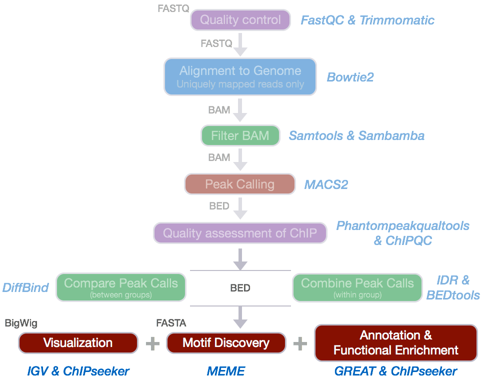
Pipeline from CD Genomics

Tool	Notes	Web address
Short-read aligners
BWA (Burrows-Wheeler Aligner)	Fast and efficient; based on the Burrows-Wheeler transform	http://bio-bwa.sourceforge.net
Bowtie	Similar to BWA, part of suite of tools that includes TopHat and CuffLinks for RNA-seq processing	http://bowtie-bio.sourceforge.net
GSNAP (Genomic Short-read Nucleotide Alignment Program)	Considers a set of variant allele inputs to better align to heterozygous sites	http://research-pub.gene.com/gmap
Wikipedia list of aligners	A comprehensive list of available short-read aligners, with descriptions and links to download the software	http://en.wikipedia.org/wiki/List_of_ sequence_alignment_software#Short- Read_Sequence_Alignment
Peak callers
MACS (Model-based Analysis for ChIP-seq)	Fits data to a dynamic Poisson distribution; works with and without control data	http://liulab.dfci.harvard.edu/MACS
PeakSeq	Takes into account differences in mappability of genomic regions; enrichment based on FDR (false-discovery rate) calculation	http://info.gersteinlab.org/PeakSeq
ZINBA (Zero-Inflated Negative Binomial Algorithm)	Can incorporate multiple genomic factors, such as mappability and GC content; can work with point-source and broad-source peak data	http://code.google.com/p/zinba

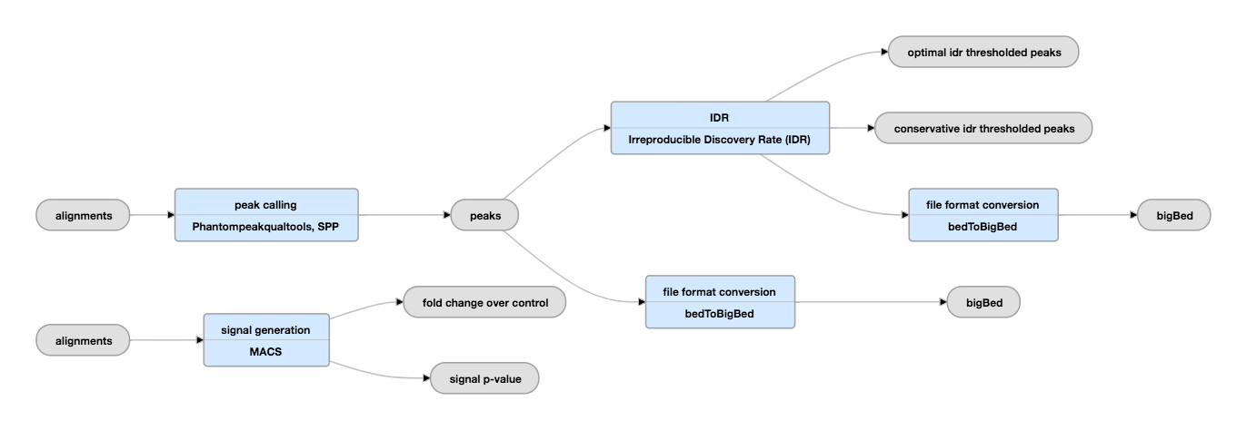
Pipeline from EncodeProject

• © ENCODE: Replicated Experiments
  

To be notice

EncodeProject list a different pipeline for treating Hitone ChiP-seq and Transcription Factor ChiP-seq.

Why different:

If you’re looking at transcription factors, then you should use a peak finder like MACS (http://liulab.dfci.harvard.edu/MACS/) to search for enrichment of your TF compared to a background samples such as input or no-ab control.
If however, you are profiling a fairly well characterised histone mark such as H3K9ac or H3K4me3 then you can simply count the reads that map near the promoters as a proxy for gene activation/repression. This can be done with Bedtools,
© Mark Ziemann, 2015

Tutorials

General Information: crazyhottommy; 2015
Tutorial from simonvh, 2018
Tutorial from IGR-lab, 2022
Tutorial from 生信技能树, 2018
Detailed Tutorial from jmzeng1314, 2018

Post analysis by R package: EpigeneticsCSAMA; 2016
More post analysis with bioconductor: brc from rockefeller edu, 2021

Example of ChiP-seq reports from commercial

• 生工生物： CHIPSEQ 项目报告.pdf
• ChIP-seq 检测报告
• 联川生物ChIP-seq 项目结题报告
• 示范ChIP-Seq结题报告

---

Part 2; Practice

A quick Tutorial from 宸宇卿

Source:

• Step1
• Step2

Environment Settel

• sra-toolkit: prepare data from NCBI

sudo apt install sra-toolkit

Data Preparation

1. Prepare directories and Dowload test data

mkdir ChiP
cd ChiP
mkdir Raw_fq

# Downlaod data with a for loop.
for ((i=593;i<601;i++)) ;do prefetch SRR1042$i ;done

# mkdir a new dir for storying our rawdata and split them into two files (Paired ends).
mv ~/ncbi/public/sra/SRR1042* Raw_fq/
cd Raw_fq

for i in $(ls);do fastq-dump --defline-seq '@$sn[_$rn]/$ri' --split-files $i; done

2. fastp to remove the header and and low quality reads and fastqc to check the quality of the reads, agian.

fastp -i in.R1.fg.gz -I in.R2.fg.g -o out.R1.fg.gz -O out.R2.fg.gz
fastqc -o outdir -t 6 out.R1.fg.gz out.R2.fg.gz

In for loop:

rm -rf *.sra
cd ..
mkdir Fastp FastQC

for i in $(ls Raw_fq/*);
    do SAMPLE=$(echo $i |awk -F"/" '{print $2}')
    fastp -i $i -o Fastp/$SAMPLE
    fastqc -o FastQC -t 6 Fastp/$SAMPLE
done

3. Reference Genome

NCBIm hg19

mkdir hg19
cd hg19

wget https://ftp.ncbi.nlm.nih.gov/genomes/all/GCF/000/001/405/GCF_000001405.40_GRCh38.p14/GCF_000001405.40_GRCh38.p14_genomic.fna.gz https://ftp.ncbi.nlm.nih.gov/genomes/all/GCF/000/001/405/GCF_000001405.40_GRCh38.p14/GCF_000001405.40_GRCh38.p14_genomic.gff.gz

bwa index GCF_000001405.40_GRCh38.p14_genomic.fna.gz
cd ..

Map the reads into reference genome

By following steps from above, you should get directories like below. Quality trimmed reads are in Fastp. Since they are single ends, we can easily align them into reference genome with less codes then paired one.

.
├── Fastp
│   ├── SRR1042593_1.fastq
│   ├── SRR1042594_1.fastq
│   ├── SRR1042595_1.fastq
│   ├── SRR1042596_1.fastq
│   ├── SRR1042597_1.fastq
│   ├── SRR1042598_1.fastq
│   ├── SRR1042599_1.fastq
│   └── SRR1042600_1.fastq
├── FastQC
├── hg19
└── Raw_fq

mkdir Bam
DB=hg19/GCF_000001405.40_GRCh38.p14_genomic.fna.gz

for i in $( ls Fastp/*);
    do SAMPLE=$(echo $i|sed 's=Fastp/==;s/_1.fastq//')
    echo $SAMPLE
    bwa mem $DB $i -t 6 |samtools view -S -b - |samtools sort > $SAMPLE.sorted.bam
    samtools index $SAMPLE.sorted.bam
    mv $SAMPE* Bam
done

Insert size.

An example of insert size for Chip-seq result.

MACS: peak calling

Documentation: macs3-project/MACS; github

pip install macs3
macs3 callpeak -t Bam/SRR1042593.sorted.bam  -c Bam/SRR1042598.sorted.bam -f BAM -g hs -n test -B -q 0.01

-g

size of the genome. It can be 1.0e+9 or 1000000000, or shortcuts:'hs' for human (2.7e9), 'mm' for mouse (1.87e9), 'ce' for C. elegans (9e7) and 'dm' for fruitfly (1.2e8), Default:hs

Results:

.
├── test_control_lambda.bdg
├── test_model.r
├── test_peaks.narrowPeak
├── test_peaks.xls
├── test_summits.bed
└── test_treat_pileup.bdg

Output Log:

INFO  @ Mon, 26 Sep 2022 11:33:39:
# Command line: callpeak -t Bam/SRR1042593.sorted.bam -c Bam/SRR1042598.sorted.bam -f BAM -g hs -n test -B -q 0.01
# ARGUMENTS LIST:
# name = test
# format = BAM
# ChIP-seq file = ['Bam/SRR1042593.sorted.bam']
# control file = ['Bam/SRR1042598.sorted.bam']
# effective genome size = 2.70e+09
# band width = 300
# model fold = [5, 50]
# qvalue cutoff = 1.00e-02
# The maximum gap between significant sites is assigned as the read length/tag size.
# The minimum length of peaks is assigned as the predicted fragment length "d".
# Larger dataset will be scaled towards smaller dataset.
# Range for calculating regional lambda is: 1000 bps and 10000 bps
# Broad region calling is off
# Paired-End mode is off

INFO  @ Mon, 26 Sep 2022 11:33:39: #1 read tag files...
INFO  @ Mon, 26 Sep 2022 11:33:39: #1 read treatment tags...
INFO  @ Mon, 26 Sep 2022 11:33:41:  1000000 reads parsed
.
.
.
INFO  @ Mon, 26 Sep 2022 11:35:12:  50000000 reads parsed
INFO  @ Mon, 26 Sep 2022 11:35:19: 50255304 reads have been read.
INFO  @ Mon, 26 Sep 2022 11:35:19: #1 tag size is determined as 51 bps
INFO  @ Mon, 26 Sep 2022 11:35:19: #1 tag size = 51.0
INFO  @ Mon, 26 Sep 2022 11:35:19: #1  total tags in treatment: 16355294
INFO  @ Mon, 26 Sep 2022 11:35:19: #1 user defined the maximum tags...
INFO  @ Mon, 26 Sep 2022 11:35:19: #1 filter out redundant tags at the same location and the same strand by allowing at most 1 tag(s)
INFO  @ Mon, 26 Sep 2022 11:35:20: #1  tags after filtering in treatment: 9821254
INFO  @ Mon, 26 Sep 2022 11:35:20: #1  Redundant rate of treatment: 0.40
INFO  @ Mon, 26 Sep 2022 11:35:20: #1  total tags in control: 50255304
INFO  @ Mon, 26 Sep 2022 11:35:20: #1 user defined the maximum tags...
INFO  @ Mon, 26 Sep 2022 11:35:20: #1 filter out redundant tags at the same location and the same strand by allowing at most 1 tag(s)
INFO  @ Mon, 26 Sep 2022 11:35:20: #1  tags after filtering in control: 47926382
INFO  @ Mon, 26 Sep 2022 11:35:20: #1  Redundant rate of control: 0.05
INFO  @ Mon, 26 Sep 2022 11:35:20: #1 finished!
INFO  @ Mon, 26 Sep 2022 11:35:20: #2 Build Peak Model...
INFO  @ Mon, 26 Sep 2022 11:35:20: #2 looking for paired plus/minus strand peaks...
INFO  @ Mon, 26 Sep 2022 11:35:23: #2 Total number of paired peaks: 5877
INFO  @ Mon, 26 Sep 2022 11:35:23: #2 Model building with cross-correlation: Done
INFO  @ Mon, 26 Sep 2022 11:35:23: #2 finished!
INFO  @ Mon, 26 Sep 2022 11:35:23: #2 predicted fragment length is 211 bps
INFO  @ Mon, 26 Sep 2022 11:35:23: #2 alternative fragment length(s) may be 211 bps
INFO  @ Mon, 26 Sep 2022 11:35:23: #2.2 Generate R script for model : test_model.r
INFO  @ Mon, 26 Sep 2022 11:35:23: #3 Call peaks...
INFO  @ Mon, 26 Sep 2022 11:35:23: #3 Pre-compute pvalue-qvalue table...
INFO  @ Mon, 26 Sep 2022 11:37:56: #3 In the peak calling step, the following will be performed simultaneously:
INFO  @ Mon, 26 Sep 2022 11:37:56: #3   Write bedGraph files for treatment pileup (after scaling if necessary)... test_treat_pileup.bdg
INFO  @ Mon, 26 Sep 2022 11:37:56: #3   Write bedGraph files for control lambda (after scaling if necessary)... test_control_lambda.bdg
INFO  @ Mon, 26 Sep 2022 11:37:56: #3   Pileup will be based on sequencing depth in treatment.
INFO  @ Mon, 26 Sep 2022 11:37:56: #3 Call peaks for each chromosome...
INFO  @ Mon, 26 Sep 2022 11:39:10: #4 Write output xls file... test_peaks.xls
INFO  @ Mon, 26 Sep 2022 11:39:10: #4 Write peak in narrowPeak format file... test_peaks.narrowPeak
INFO  @ Mon, 26 Sep 2022 11:39:10: #4 Write summits bed file... test_summits.bed
INFO  @ Mon, 26 Sep 2022 11:39:10: Done!

Visual

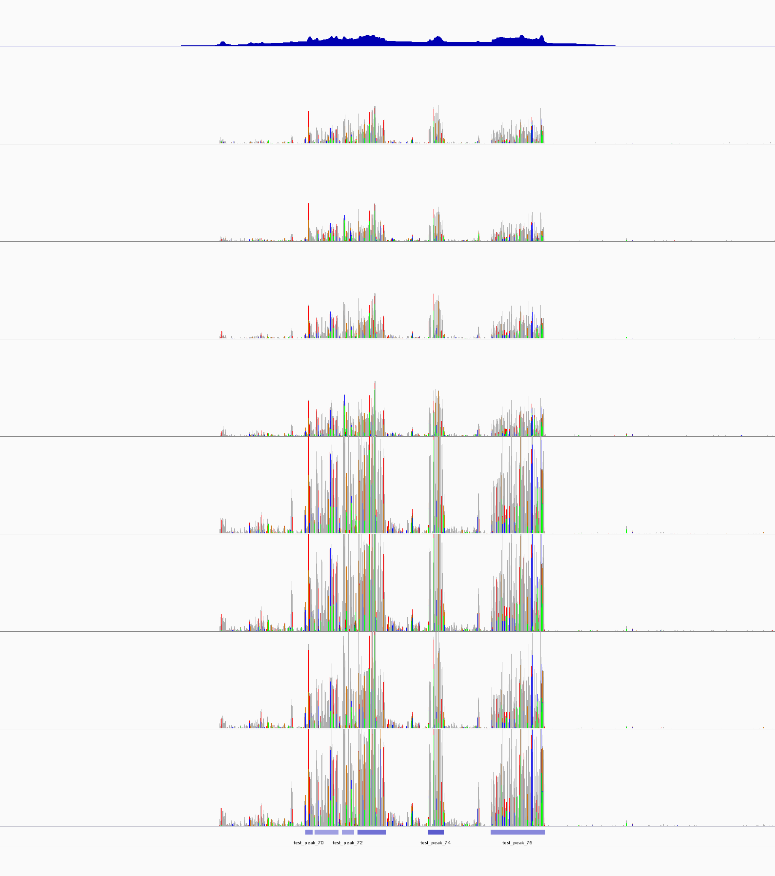
IGV

The peak(s) with the best Pvalue. The first track is test_control_lambda.bdg file. the last track is from test_peaks.narrowPeak file. The color of each bar seems corrosponded the P-value. The 5th peak has the lowest p-value and the darkest blue.

An example of Unreliable peak. Tow peaks were called based on 3th and 5th but can not be found between 4th and 6th which are biological repeats.

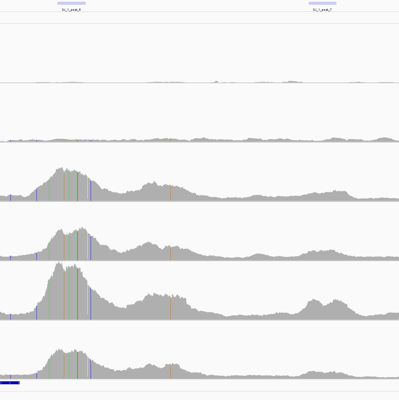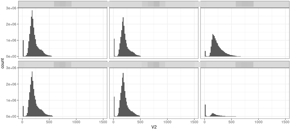
ggplot

samtools depth Bam/SRR1042593.sorted.bam > SRR1042593.csv
samtools depth Bam/SRR1042598.sorted.bam > SRR1042598.csv

library(ggplot2)
A <- read.table("SRR1042593.csv")
A$Sample = "SRR1042593"
B <- read.table("SRR1042598.csv")
B$Sample = "SRR1042598"

TB <- rbind(A,B)
BED <- read.table("test_peaks.xls", header=T)

TMP<-TB[TB$V2 %in% c(
.9*BED$start[BED$X.log10.pvalue==max(BED$X.log10.pvalue)]
:1.1*BED$end[BED$X.log10.pvalue==max(BED$X.log10.pvalue)),]


TMP <- TB[TB$V2>= BED$start[BED$X.log10.pvalue==max(BED$X.log10.pvalue)],]
TMP <- TMP[TMP$V2<= BED$end[BED$X.log10.pvalue==max(BED$X.log10.pvalue)],]

ggplot(TMP, aes(V2, V3)) + geom_bar(stat = 'identity') + facet_grid(~Sample)

After Peak calling

There is a pipeline

echo hello wold

hello wold