String DB

String Database

Download Specious Network

Link to downloading the networks

An example of download files:

• Link file: 7227.protein.physical.links.full.v11.5.txt
• Protein annotation: 7227.protein.info.v11.5.txt.gz

TB <- read.table("7227.protein.links.detailed.v11.5.txt", header = T)

dim(TB)
str(TB)

[1] 4343798      10

'data.frame':	4343798 obs. of  10 variables:
 $ protein1      : chr  "7227.FBpp0070001" "7227.FBpp0070001" "7227.FBpp0070001" "7227.FBpp0070001" ...
 $ protein2      : chr  "7227.FBpp0293850" "7227.FBpp0087873" "7227.FBpp0079990" "7227.FBpp0080090" ...
 $ neighborhood  : int  0 0 0 0 0 0 0 0 0 0 ...
 $ fusion        : int  0 0 0 0 0 0 0 0 0 0 ...
 $ cooccurence   : int  0 0 0 0 0 0 0 0 0 0 ...
 $ coexpression  : int  151 153 167 298 446 371 242 371 373 238 ...
 $ experimental  : int  0 0 0 0 0 0 0 0 0 0 ...
 $ database      : int  0 0 0 0 0 0 0 0 0 0 ...
 $ textmining    : int  0 0 0 0 0 0 0 0 0 0 ...
 $ combined_score: int  150 152 167 298 446 371 241 371 373 237 ...

• Protein 1: Start protein
• Protein 2: Connections from Protein 1 to protein 2
• neighborhood: Physical neighborhood on the Genome
• fusion: raw fusion score for COG mode (deprecated).
• cooccurence: raw cooccurence score for COG mode (deprecated).
• coexpression: expression patterns in a group of RNA-Seq are similar
• experimental: experimental score (derived from experimental data, such as, affinity chromatography).
• database: database score (derived from curated data of various databases).
• textmining: textmining score (derived from co-occurring mentioning of gene/protein names in abstracts).
• combined_score: scores in total

From:

• Table: network.score_types
• Starting Point

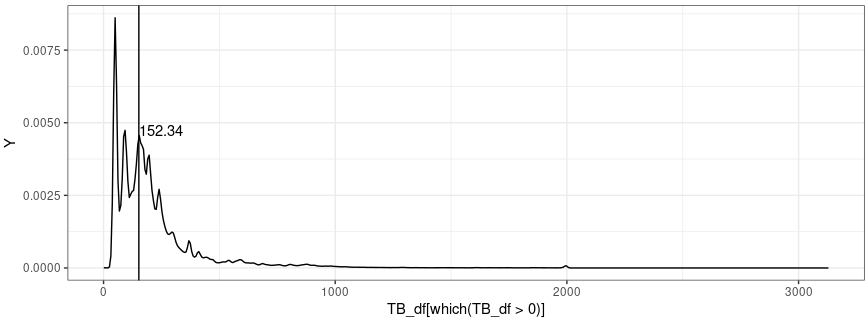
How do I select a reasonable score cut-off value for my analysis?

You can use the score cut-off to limit the number of interactions to those that have higher confidence and are more likely to be true positives. Setting the cutoff lower will increase coverage but also a fraction of false positives. You have to choose some arbitrary number based on the number of interactions you need for your analysis.

What is co-occurrence

A type of phylogenetic profile – the patterns of the presence or absence of orthologs across many organisms© Pan-Jun Kim, 2011

Example in R

library(ggplot2)
library(stringr)
library(igraph)
library(reshape2)

Anno <-  read.csv("7227.protein.info.v11.5.txt", sep ='\t', header = T, quote = "")
Anno[[1]] <- str_remove(Anno[[1]], "7227.")

TB <- read.table("7227.protein.links.detailed.v11.5.txt", header = T)
TB2 <- TB[c("protein1", "protein2", "fusion", "cooccurence", "coexpression", "experimental")]
TB2$protein1 <- str_remove(TB2$protein1, "7227.")
TB2$protein2 <- str_remove(TB2$protein2, "7227.")

TB_df <- apply(TB2[-c(1:2)], 1, sum)

N = 18+ which.max(density(TB_df[which(TB_df>0)])$y[-c(1:18)])
X = density(TB_df[which(TB_df>0)])$x[N]
Y = density(TB_df[which(TB_df>0)])$y[N]

ggplot() + geom_density(aes(x= TB_df[which(TB_df>0)])) + theme_bw() +
    geom_vline(xintercept =  X) +
    geom_text(aes(x= X, y = Y, label= round(X, 2)), hjust = 0, vjust = 0)

# LIST

LIST <- c("FBpp0070483", "FBpp0288697", "FBpp0304573", "FBpp0305946", "FBpp0300852", "FBpp0083503", "FBpp0297544", "FBpp0085082", "FBpp0288660", "FBpp0077739", "FBpp0081139", "FBpp0293081", "FBpp0079676", "FBpp0288515", "FBpp0297890", "FBpp0304299", "FBpp0306192", "FBpp0074686", "FBpp0070417", "FBpp0086911", "FBpp0289616")

# Try threshold at 2000
# TB3 <- TB2[which(TB_df>1000),]
TB3 <- rbind(TB2[TB2$protein1 %in% LIST,], TB2[TB2$protein2 %in% LIST,])
TB_df <- apply(TB3[-c(1:2)], 1, sum)
TB3 <- TB3[which(TB_df>150),]
length(unique(c(TB3$protein1, TB3$protein2 )))
# 173; we have 173 unique proteins


# plot it with igraph
TB3$CN = 1
TB4 <- reshape(TB3[c("protein1", "protein2", "CN")], idvar = "protein1", timevar = "protein2", direction = "wide")
rownames(TB4) <- TB4[[1]]
TB4 <- TB4[-1]
colnames(TB4) <- str_remove(colnames(TB4), "CN.")
TB4[is.na(TB4)] <- 0

network=graph_from_adjacency_matrix(as.matrix(TB4) , mode='undirected', diag=T )

TB4.Size <- as.data.frame(table(c(TB3$protein1, TB3$protein2 )))
TB4.Size <- TB4.Size[match(colnames(TB4),TB4.Size$Var1),]
TB4.Size$Anno <- Anno[[2]][match(TB4.Size$Var1,Anno[[1]])]
TB4.Size$Anno2 = ""
TB4.Size$Anno2[which(TB4.Size$Freq>=100)] <- TB4.Size$Anno[which(TB4.Size$Freq>=100)]
##DefauTB4.Size$Anno2 = ""
set.seed(1)
par(mar=c(0,0,0,0))
plot(network,    
    vertex.size= log(TB4.Size$Freq +1),
    vertex.label = TB4.Size$Anno2 ,
    vertex.label.size= log(TB4.Size$Freq +1) ,
    vertex.frame.color= adjustcolor("salmon", alpha.f = .5),
    vertex.color = adjustcolor("salmon", alpha.f = .5),
    edge.color = adjustcolor("grey", alpha.f = .1), layout = layout_nicely)

lay = layout_with_graphopt(network)
R = max(abs(lay))
lay_Y = abs(asin(sin(lay[,2]/sqrt(lay[,1]^2 + lay[,2]^2))) * R)
lay_X = abs(acos(cos(lay[,1]/sqrt(lay[,1]^2 + lay[,2]^2))) * R)
lay_X[lay[,1]<0] <- lay_X[lay[,1]<0] * -1
lay_Y[lay[,2]<0] <- lay_Y[lay[,2]<0] * -1

LX <- 2*(lay_X -lay[,1]) #+ lay[,1]
LY <- 2*(lay_Y -lay[,2]) #+ lay[,2]

LAY <- matrix(c(LX, LY) , ncol = 2)
#layout_with_mds
#layout_nicely
#layout_with_graphopt