From igraph to ggplot2
Turn igraph result to ggplot2 plot
Why you want to turn igraph network polot to ggplot?
- Flexibility: ggplot is a very flexible and customizable plotting package that allows you to create high-quality, publication-ready plots with a high degree of control over the visual aesthetics of your plots. You can easily modify various aspects of the plot, such as the color, shape, and size of the nodes and edges, and the placement of the labels.
- Integration with igraph: ggplot works seamlessly with igraph, making it easy to create complex and informative visualizations of your network data. You can use ggplot to visualize network data in a variety of ways, including heatmaps, scatterplots, and bar charts.
- Consistency: ggplot provides a consistent grammar for building plots, which makes it easy to create plots with a consistent style and look across different datasets. This can be particularly useful if you are working with multiple datasets and want to create a consistent visual language for your plots.
- Reproducibility: ggplot produces code that can be easily reproduced, making it easier to share and collaborate on your work. You can also easily modify and update your plots as your data or analysis changes. Overall, using ggplot to plot igraph results can help you create informative, visually appealing, and reproducible visualizations of your network data.
Basic idea of this post is from © Christopher Chizinski, 2014. It is an old post but all codes work just fine!
install igraph
|
-
Errors
libopenblas.so.0: cannot open shared object file: No such file or directory
sudo apt-get install libopenblas-dev
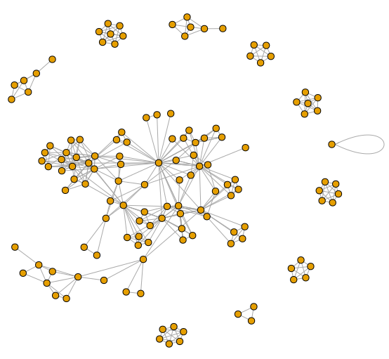
Example data for igraph
|
|
 |
 |
|---|
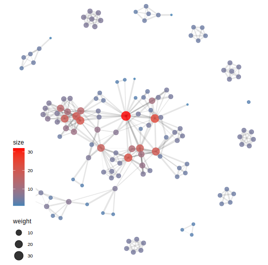
include size of the dots and the weight of edges
|
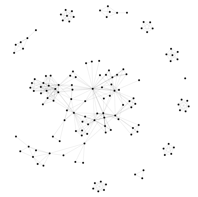
From igraph to ggplot2


