path find in a network plot

path find in a network plot

Here’s an example code for a more complicated network graph using NetworkX and finding a path from one node to another node:

import networkx as nx
import matplotlib.pyplot as plt

# Create a graph
G = nx.DiGraph()

# Add nodes
G.add_nodes_from(['A', 'B', 'C', 'D', 'E', 'F', 'G', 'H'])

# Add edges
G.add_edges_from([('A', 'B'), ('B', 'C'), ('B', 'D'), ('C', 'E'), ('D', 'E'),
                  ('D', 'F'), ('E', 'G'), ('F', 'G'), ('G', 'H')])

# Plot the graph
pos = nx.spring_layout(G, seed=123)
nx.draw_networkx(G, pos, with_labels=True)
edge_labels = nx.get_edge_attributes(G, 'weight')
nx.draw_networkx_edge_labels(G, pos, edge_labels=edge_labels)
plt.show()

# Find a path from node 'A' to node 'H'
path = nx.shortest_path(G, 'A', 'H')
print(path)


# highlight the path
edge_colors = ['red' if (u, v) in zip(path, path[1:]) else 'black' for u, v in G.edges()]
nx.draw(G,  pos, with_labels=True, edge_color=edge_colors)
plt.show()

['A', 'B', 'C', 'E', 'G', 'H']

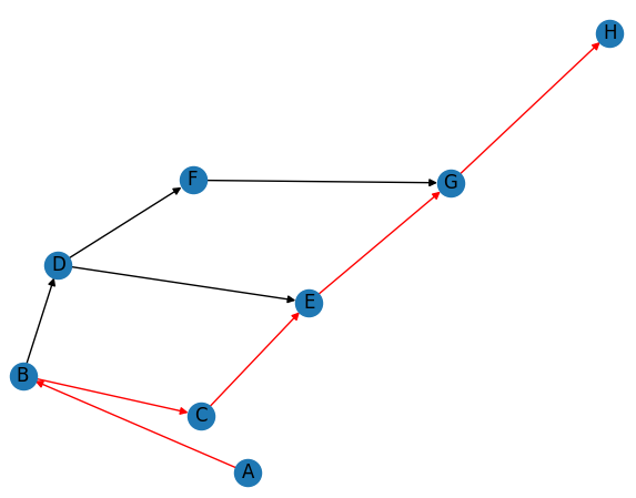
In this code, we create a directed graph G using nx.DiGraph(). We add nodes to the graph using G.add_nodes_from(), and add edges to the graph using G.add_edges_from(). We can assign a weight to each edge using a dictionary, but in this example we don’t do that.

We then use the nx.spring_layout() function to generate node positions for the graph. This function positions nodes using the Fruchterman-Reingold force-directed algorithm. In this example, we set the random seed to 123 using the seed parameter of nx.spring_layout(). This ensures that the initial conditions of the spring layout algorithm are the same each time you run the code, and the layout of the graph remains the same.

We then use nx.draw_networkx() to draw nodes and edges of the graph with labels. We also use nx.get_edge_attributes() and nx.draw_networkx_edge_labels() to add labels to the edges of the graph. Finally, we use plt.show() to display the plot.

After displaying the graph, we use nx.shortest_path() to find the shortest path from node ‘A’ to node ‘H’. The function returns a list of nodes that form the path. We print the path to the console.

Note that you can modify the graph and the path-finding algorithms according to your specific needs using the functions available in the NetworkX library.

How does nx.shortest_path works

The nx.shortest_path() function in NetworkX is used to find the shortest path between two nodes in a graph. It uses the Dijkstra’s algorithm, which is an algorithm for finding the shortest paths between nodes in a graph.

The nx.shortest_path() function takes three parameters:

• G: the graph to search for shortest path in.
• source: the starting node for the path.
• target: the ending node for the path.
  The function returns a list of nodes in the shortest path from the source node to the target node.

what is Dijkstra’s algorithm

Dijkstra’s algorithm is a graph search algorithm that works by finding the shortest path from a starting node to all other nodes in the graph. The algorithm maintains a set of visited nodes and a set of unvisited nodes, with the distance from the starting node to each unvisited node initialized to infinity. At each step, the algorithm selects the unvisited node with the smallest distance from the starting node and adds it to the visited set. It then updates the distances of all adjacent nodes that are still in the unvisited set, setting their distance to the sum of the distance to the current node and the weight of the edge between them. The algorithm continues until the target node is reached, or until all nodes have been visited.

Once the shortest path has been found, nx.shortest_path() returns a list of nodes in the path, in the order that they appear in the path.

What is “bellman-ford”?

Bellman-Ford is an algorithm for finding the shortest paths between nodes in a weighted graph. The algorithm can handle negative edge weights, whereas Dijkstra’s algorithm, which we discussed in a previous question, cannot. However, Bellman-Ford is slower than Dijkstra’s algorithm and has a higher time complexity of O(V*E), where V is the number of vertices and E is the number of edges in the graph.

The Bellman-Ford algorithm works by relaxing all edges in the graph V-1 times, where V is the number of vertices in the graph. During each iteration, the algorithm checks if the distance to a node can be improved by going through another node. If so, it updates the distance to the node. The algorithm repeats this process V-1 times to ensure that all possible paths have been explored.

After the V-1 iterations, the algorithm performs one more check to see if there are any negative weight cycles in the graph. If there are, then the algorithm cannot find a shortest path because the distance to the node can be decreased indefinitely by traversing the negative cycle. In this case, the algorithm returns a message indicating that a negative cycle has been detected.

import networkx as nx

# Create a graph
G = nx.DiGraph()

# Add nodes
G.add_nodes_from(['A', 'B', 'C', 'D', 'E'])

# Add edges with weights
G.add_weighted_edges_from([('A', 'B', 3), ('A', 'C', 8), ('B', 'C', -4),
                           ('B', 'D', 1), ('B', 'E', 7), ('C', 'D', 2),
                           ('D', 'B', 2), ('E', 'D', -5)])

# Find the shortest paths using Bellman-Ford algorithm
distances, predecessors = nx.bellman_ford(G, 'A')

# Print the distances
print(distances)

# Print the predecessors
print(predecessors)

In this example, we create a directed graph with five nodes and eight edges, with some edges having negative weights. We then use nx.bellman_ford() to find the shortest paths from the node ‘A’ to all other nodes in the graph. The function returns two dictionaries: one with the shortest distance from the starting node to each node, and another with the predecessor node in the shortest path for each node. We print these dictionaries to the console.