AI: Logistic Regression

Logistic Regression

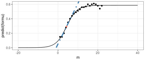
Logistic regression is a supervised machine learning algorithm used for binary classification tasks. Unlike linear regression, which predicts continuous values, logistic regression predicts the probability that a given input belongs to a certain class.

Key Concepts in Logistic Regression

1. Logistic Function (Sigmoid Function):

   • Logistic regression uses the sigmoid function to map predicted values to probabilities:
     $$
     \sigma(z) = \frac{1}{1 + e^{-z}}
     $$
     • $ z = X \beta $: Linear combination of features.
     • The output of $ \sigma(z) $ is always between 0 and 1, representing the probability.

2. Logit Link Function:

   • The logit function is the natural logarithm of the odds (log-odds) of the binary outcome:
     $$
     g(\theta) = \log\left(\frac{P(y=1|X)}{P(y=0|X)}\right)
     $$
   • It transforms probabilities into log-odds:
     $$
     g(\theta) = X^T\beta
     $$

3. Inverse Link Function:

   • To map the log-odds ($ X^T\beta $) back to probabilities, we use the inverse of the logit function:
     $$
     P(y=1|X, \beta) = \frac{e^{XT\beta}}{1 + e^{XT\beta}}
     $$
     • This is the sigmoid function, which outputs probabilities between 0 and 1.

4. Decision Boundary:

   • For binary classification:
     • If $ \sigma(z) \geq 0.5 $, classify the input as Class 1.
     • If $ \sigma(z) < 0.5 $, classify the input as Class 0.

5. Log-Likelihood:

   • Logistic regression optimizes the log-likelihood instead of minimizing residuals (like in linear regression):
     $$
     \ell(\beta) = \sum_{i=1}^n \left[ y_i \ln(\hat{y}_i) + (1 - y_i) \ln(1 - \hat{y}_i) \right]
     $$
     Where:
     • $ \hat{y}_i = \sigma(z_i) $: Predicted probability.
     • $ y_i $: Actual class (0 or 1).

6. Negative Log-Likelihood:

   • The optimization process in machine learning (and statistics) often involves minimizing a cost function. Since the log-likelihood is a measure of fit (higher is better), we take its negative to convert the maximization problem into a minimization problem:
   • $$ -\ln L(\beta) = -\sum_{i=1}^n \left[ y_i X_i^T \beta - \ln(1 + e^ {X_i^ T \beta}) \right] $$

7. Optimization:

   • The goal is to find the coefficients $ \beta $ that maximize the log-likelihood using algorithms like Gradient Descent or Newton’s Method.

What is a Link Function?

A link function connects the linear predictor ($ X\beta $) to the mean of the response variable in a generalized linear model (GLM). It provides a transformation that ensures the predicted values from the model stay within the valid range for the response variable.

Why negative Log-likelihood function?

• The negative log-likelihood is used to simplify optimization by turning a maximization problem into a minimization one.
• The formula on the slide and in my explanation are equivalent, just written in slightly different forms.

Applications of Logistic Regression

• Binary classification problems such as:
  • Email spam detection (Spam/Not Spam).
  • Disease diagnosis (Positive/Negative).
  • Customer churn prediction (Churn/No Churn).

Practical Example: Binary Classification with Logistic Regression

Below is a Python example using scikit-learn:

Problem: Predict whether a person has heart disease based on two features.

from sklearn.datasets import make_classification
from sklearn.linear_model import LogisticRegression
from sklearn.model_selection import train_test_split
from sklearn.metrics import accuracy_score, confusion_matrix, classification_report
import matplotlib.pyplot as plt

# Generate synthetic binary classification dataset
X, y = make_classification(n_samples=200, n_features=2, n_informative=2, n_redundant=0, random_state=42)

# Split the dataset into training and testing sets
X_train, X_test, y_train, y_test = train_test_split(X, y, test_size=0.3, random_state=42)

# Fit logistic regression model
model = LogisticRegression()
model.fit(X_train, y_train)

# Make predictions
y_pred = model.predict(X_test)

# Evaluate the model
accuracy = accuracy_score(y_test, y_pred)
print("Accuracy:", accuracy)
print("Confusion Matrix:\n", confusion_matrix(y_test, y_pred))
print("Classification Report:\n", classification_report(y_test, y_pred))

# Plot decision boundary
import numpy as np
x_min, x_max = X[:, 0].min() - 1, X[:, 0].max() + 1
y_min, y_max = X[:, 1].min() - 1, X[:, 1].max() + 1
xx, yy = np.meshgrid(np.arange(x_min, x_max, 0.1),
                     np.arange(y_min, y_max, 0.1))
Z = model.predict(np.c_[xx.ravel(), yy.ravel()])
Z = Z.reshape(xx.shape)

plt.contourf(xx, yy, Z, alpha=0.8)
plt.scatter(X[:, 0], X[:, 1], c=y, edgecolor='k', marker='o')
plt.title("Logistic Regression Decision Boundary")
plt.xlabel("Feature 1")
plt.ylabel("Feature 2")
plt.show()

Logistic Regression for Multiclass Classification

Logistic regression can be extended to handle multiclass classification problems where the target variable has more than two classes. The two common approaches are One-vs-Rest (OvR) and Softmax (Multinomial) logistic regression.

One-vs-Rest (OvR)

Overview:

• In OvR, a separate binary classifier is trained for each class.
• For a class $ k $, the classifier treats:
  • $ y = k $ as positive (1).
  • $ y \neq k $ as negative (0).
• Each classifier predicts the probability of the input belonging to its class.

Prediction:

• For a new data point, the class with the highest probability is chosen:
  $$
  \hat{y} = \arg\max_{k} P(y = k | x)
  $$

Softmax (Multinomial) Logistic Regression

Softmax logistic regression generalizes binary logistic regression to multiple classes. Instead of fitting separate binary classifiers, it predicts the probability for all classes simultaneously using the softmax function.

Softmax Function:

$$
P(y = k | x) = \frac{e^{X \beta_k}}{\sum_{j=1}^K e^{X \beta_j}}
$$
Where:

• $ K $: Total number of classes.
• $ \beta_k $: Coefficients for class $ k $.
• $ P(y = k | x) $: Probability of class $ k $ given the input $ x $.

Prediction:

• For a new data point, the class with the highest softmax probability is chosen:
  $$
  \hat{y} = \arg\max_{k} P(y = k | x)
  $$

Summary of Methods:

Method	When to Use	Advantages	Disadvantages
One-vs-Rest	Small datasets with a limited number of classes.	Easy to implement, interpretable.	Can struggle with overlapping classes.
Softmax	When normalized probabilities across classes are needed.	Probabilities are calibrated.	Computationally expensive.

Softmax approach (also called multinomial logistic regression)

1. C-Class Classification:

   • The goal is to classify the target variable $ y $ into one of $ C $ classes:
     $$
     y \in {0, 1, \dots, C-1}
     $$

2. Discrete Probability Distribution:

   • The probabilities $ \theta_0, \theta_1, \dots, \theta_{C-1} $ represent the likelihood of a data point belonging to each class.
   • These probabilities satisfy:
     $$
     \theta_i \in [0, 1] \quad \text{and} \quad \sum_{i=0}^{C-1} \theta_i = 1
     $$

3. Link Function:

   • The relationship between the linear model ($ X\beta $) and the class probabilities is established using the Softmax function:
     $$
     g(\theta) = \log \left( \frac{\theta_i}{1 - \sum_{u=0}^{C-1} \theta_u} \right) = X^T \beta
     $$

4. Class Probabilities:

   • For each class $ i $, the probability is computed as:
     $$
     P(y = i | X, \beta) = \frac{e^ {X^ T \beta_i}}{1 + \sum_{j=0}^ {C-1} e^ {X^ T \beta_j}}
     $$
   • For the last class $ C-1 $, the probability is:
     $$
     P(y = C-1 | X, \beta) = \frac{1}{1 + \sum_{i=0}^{C-2} e^ {X^T \beta_i}}
     $$