KEGG result visualization by ggplot

KEGG result visualization by ggplot

用ggplot画KEGG结果

Data

Before running the codes, I’d like to have a brief introduces about my data.

As you can see codes below, List has all files I need.
Take Intest_30_vs_Intest_75 as an example:

#KEGGid	KEGGdescription	KEGGclass	KEGGsubclass	Oddsratio	p-value	q-value	Gene_numbers
04610	Complement and coagulation cascades	Organismal Systems	Immune system	11.7158541941	6.30141083687e-10	1.18731846295e-07	14
04977	Vitamin digestion and absorption	Organismal Systems	Digestive system	11.1739766082	0.000269773611998	0.0254155139724	5
04974	Protein digestion and absorption	Organismal Systems	Digestive system	3.73319892473	0.000445170135803	0.0279598085294	11

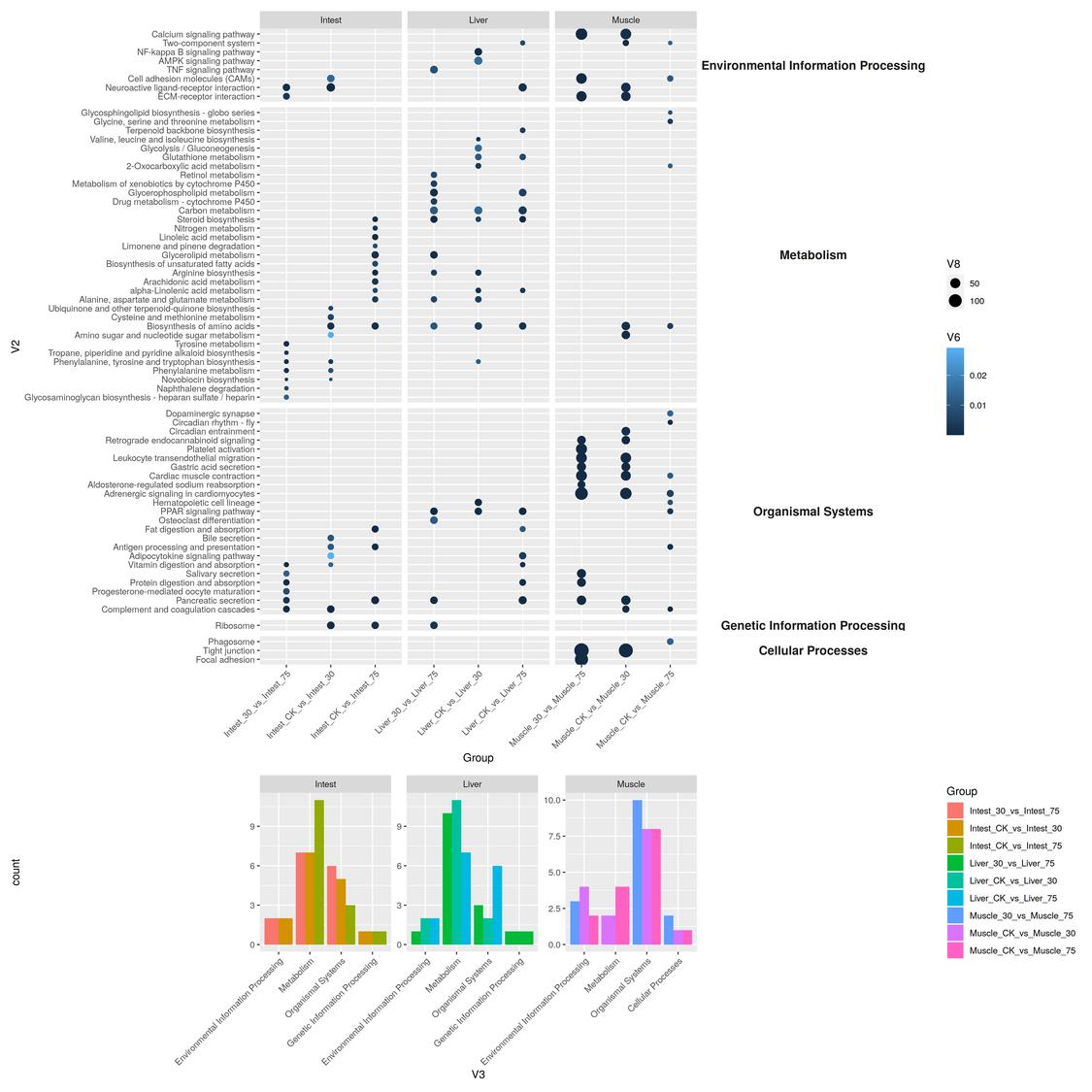
Quick Start

library(ggplot2)
library(reshape2)
library(patchwork)

List = c('Intest_30_vs_Intest_75','Intest_CK_vs_Intest_30','Intest_CK_vs_Intest_75','Liver_30_vs_Liver_75','Liver_CK_vs_Liver_30','Liver_CK_vs_Liver_75','Muscle_30_vs_Muscle_75','Muscle_CK_vs_Muscle_30','Muscle_CK_vs_Muscle_75')

TB = data.frame()

for(i in List){
  A <- read.table(paste("../",i,"/kegg_annotation/Diff_exprs.KEGG_enrich.lst.network", sep = ""), sep = '\t')
  A$Group=i
  print(dim(A))
  TB = rbind(TB,A)
}

TB$SubG = "Intest"
TB$SubG[grep( "Muscle", TB$Group)] = "Muscle"
TB$SubG[grep( "Liver", TB$Group)]  = "Liver"
## KEGG Dots
p1<- ggplot(TB)+ geom_point(aes(x=Group,y=V2,size=V8,color=V6)) +
     theme(axis.text.x =  element_text(angle = 45,hjust = 1)) +
     facet_grid(~SubG, scales = 'free')

p2 <- ggplot(TB)+ geom_point(aes(x=Group,y=V2,size=V8,color=V6)) +
      theme(axis.text.x =  element_text(angle = 45,hjust = 1), strip.text.y = element_text(size=12, face="bold", angle = 0), strip.background.y = element_blank())  +
      facet_grid(V3~SubG, scales = 'free', space = 'free')

p3 <- ggplot(TB)+ geom_point(aes(x=Group,y=V2,size=V8,color=V6)) +
      theme(axis.text.x =  element_text(angle = 45,hjust = 1), strip.text.y = element_text(size=12, face="bold", angle = 0), strip.background.y = element_blank())  +
      facet_grid(V4~SubG, scales = 'free', space = 'free')


## KEGG subclass_bar
p4 <- ggplot(TB)+ geom_bar(aes(x=V3,fill=Group), ,position = 'dodge') +
      theme(axis.text.x =  element_text(angle = 45,hjust = 1))+
      facet_wrap(~SubG, scales = 'free')
LL <- 'A
A
A
A
B'
p2+p4  +plot_layout(design = LL)

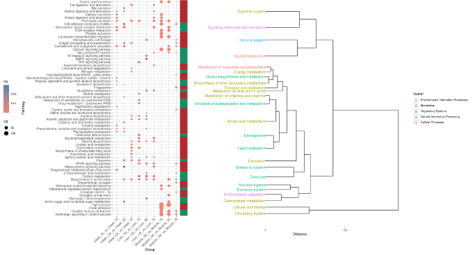
More complicate plot

Functions TreePlot and LS_judg could be found at: Blog/Yueque

clust_TB <- reshape(TB[c("V4","V8","Group")],timevar='Group', idvar=c('V4'),direction='wide')
row.names(clust_TB)=clust_TB[[1]]
clust_TB= clust_TB[-1]
clust_TB[is.na(clust_TB)] = 0

hc <- hclust(dist(clust_TB))
dendr    <- dendro_data(hc, type="rectangle") # convert for ggplot
dendr$labels$cluster <- TB$V3[match(dendr$labels$label,TB$V4)]
## plot the dendrogram; note use of color=cluster in geom_text(...)
p_tree <- ggplot() +
  geom_segment(data=segment(dendr), aes(x=x, y=y, xend=xend, yend=yend)) +
  geom_text(data=label(dendr), aes(x, y, label=label, hjust=0, color=cluster),
           size=3) +
  coord_flip() + #scale_y_reverse(expand=c(0.2, 0)) +
  theme(axis.line.y=element_blank(),
        axis.ticks.y=element_blank(),
        axis.text.y=element_blank(),
        axis.title.y=element_blank(),
        panel.background=element_rect(fill="white"),
        panel.grid=element_blank())

TB$V4 = factor(TB$V4,levels(dendr$labels$label))
TB = TB[order(TB$V4),]
TB$V2 = factor(TB$V2,levels=(unique(TB$V2)))

TB_mbar = data.frame(table(unique(TB[c("V2","V4")])$V4))
TB_mbar$hei = TB_mbar$Freq[1]/2
for(i in c(2:nrow(TB_mbar))){
  TB_mbar$hei[i] =sum(TB_mbar$Freq[1:i-1])+ (TB_mbar$Freq[i]/2)
}
Width_tree = TB_mbar$hei
den_2 <- TreePlot(dendr, Width_tree)

Result = c()
C_list=c('#178c60','#B4292C')
TB_mbar = data.frame(table(TB$V4))
Num = 0
for(i in TB_mbar$Freq){
  Result = c(Result,rep(C_list[Num%%2+1],i))
  Num = Num +1
}

p_dot <- ggplot(TB)+ geom_point(aes(x=Group,y=V2,size=V8,color=V6)) +
              labs(y="Pathway")+
              theme(axis.text.x =  element_text(angle = 45,hjust = 1),
                axis.text = element_text(size=10),
                strip.text.y = element_text(size=12, face="bold", angle = 0),
                strip.background.y = element_blank(),
                legend.position='left',
                panel.background = element_blank(),
                panel.grid.major= element_line(linetype=2,color='grey'),   
                panel.grid.minor= element_blank())+   
              geom_tile(aes(x=10,y=V2), fill= Result)+
              scale_color_gradient(low = "salmon",high = "steelblue")

p_tree <- ggplot() +
          geom_segment(data=segment(den_2), aes(x=x, y=y, xend=xend,
            yend=yend)) +
          geom_text(data=label(dendr), aes(Width_tree, y,
            label=levels(dendr$labels$label), hjust=1,
            color=cluster),size=4) +
          coord_flip() + #scale_y_reverse(expand=c(0.2, 0)) +
          labs(y='Distance')+
          theme(axis.line.y=element_blank(),
            axis.ticks.y=element_blank(),
            axis.text.y=element_blank(),
            axis.title.y=element_blank(),
            panel.background=element_blank(),
            panel.grid=element_blank()) + expand_limits(y=c(-80,10),x=c(0,68))

ggdraw() + draw_plot(p_dot,0,0.007,0.4)+  
           draw_plot(p_tree,0.4,0.068,0.6,0.98)

ggsave('KEGG_tree.png',wi=20.4,hei=11)

More

Get a KEGG results first

codes from: ClusterProfiler

library(clusterProfiler)

data(geneList, package="DOSE")
gene <- names(geneList)[abs(geneList) > 2]

kk <- enrichKEGG(gene         = gene,
                 organism     = 'hsa',
                 pvalueCutoff = 0.05)
head(kk)

$Cos\alpha = \frac{tA}{tC}$
$Sin\alpha = \frac{\sqrt{tC^2 - tA^2}}{tC}$
$mC = \frac{mB_1}{Sin\alpha}$
$mtC = mC * \frac{mB_1 - mB_2}{mB_2}$
$S = mtC/tC$
$S = \frac{mC * \frac{mB_1 - mB_2}{mB_2}}{tC}$
$S = \frac{\frac{mB_1}{Sin\alpha} * \frac{mB_1 - mB_2}{mB_2}}{tC}$
$S = \frac{\frac{mB_1}{\frac{\sqrt{tC^2 - tA^2}}{tC}} * \frac{mB_1 - mB_2}{mB_2}}{tC}$
$S = \frac{\frac{mB_1}{\frac{\sqrt{tC^2 - tA^2}}{tC}} * \frac{mB_1 - mB_2}{mB_2}}{tC}$
$S = \frac{\frac{mB_1^2 - mB_1 * mB_2 }{\frac{mB_2\sqrt{tC^2 - tA^2}}{tC}}}{tC}$
$S = \frac{mB_1^2 - mB_1 * mB_2 }{\frac{mB_2\sqrt{tC^2 - tA^2}}{tC2}}$
$S = \frac{mB_1^2 - mB_1 * mB_2 }{tC^2 * mB_2\sqrt{tC^2 - tA^2}}$