Reading ab1 file with R

Reading ab1 file with R (sangerseqR)

Install: Bioconductor
ReadMe: PDF

Install

if (!requireNamespace("BiocManager", quietly = TRUE))
    install.packages("BiocManager")

BiocManager::install("sangerseqR")

Quick Start

library(sangerseqR)

A <- read.abif("119DOWN-ST.119DOWN-F.11731873.C04.ab1")
str(A)

Formal class 'abif' [package "sangerseqR"] with 3 slots
  ..@ header   :Formal class 'abifHeader' [package "sangerseqR"] with 9 slots
  .. .. ..@ abif       : chr "ABIF"
  .. .. ..@ version    : int 101
  .. .. ..@ name       : raw [1:4] 74 64 69 72
  .. .. ..@ number     : int 1
  .. .. ..@ elementtype: int 1023
  .. .. ..@ elementsize: int 28
  .. .. ..@ numelements: int 118
  .. .. ..@ dataoffset : int 259806
  .. .. ..@ datahandle : int 0
  ..@ directory:Formal class 'abifDirectory' [package "sangerseqR"] with 7 slots
  .. .. ..@ name       : chr [1:118] "AEPt" "AEPt" "APFN" "APXV" ...
  .. .. ..@ tagnumber  : int [1:118] 1 2 2 1 1 1 1 1 1 1 ...
  .. .. ..@ elementtype: int [1:118] 4 4 18 19 19 19 2 5 4 4 ...
  .
  .
  .

Data

Electronic Signal Matrix

A@data$DATA.1
A@data$DATA.2
A@data$DATA.3
A@data$DATA.4

Base Signal Matrix

A@data$DATA.9
A@data$DATA.10
A@data$DATA.11
A@data$DATA.12

Plot

library(ggplot2)

Y1 = head(A@data$DATA.9,3000)
Y2 = head(A@data$DATA.10,3000)
Y3 = head(A@data$DATA.11,3000)
Y4 = head(A@data$DATA.12,3000)

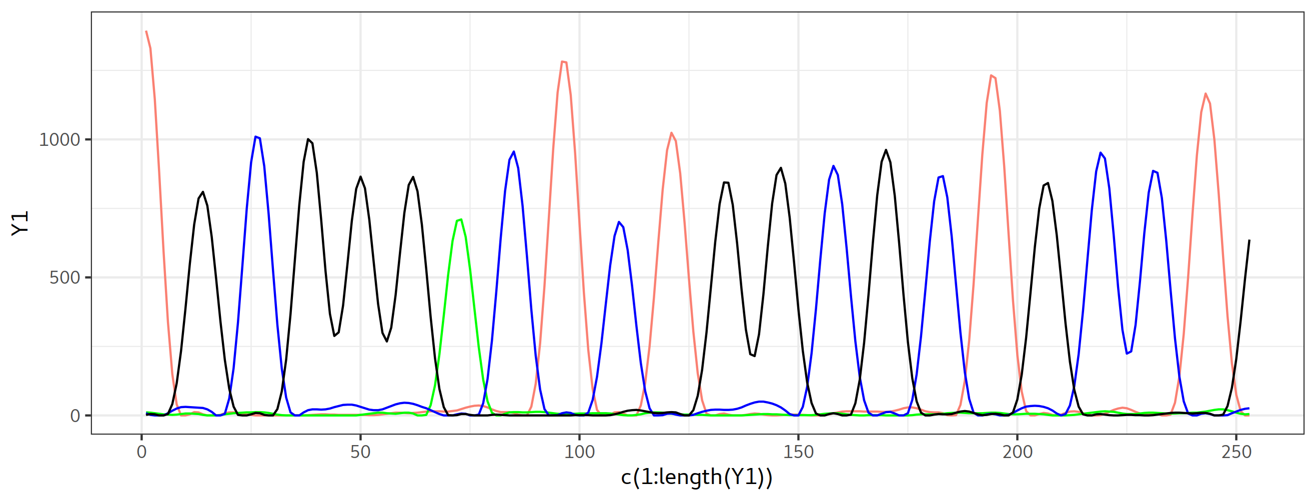
ggplot() + geom_path(aes(x=c(1:length(Y1)), y= Y1),color='salmon')+
  geom_path(aes(x=c(1:length(Y2)), y= Y2),color='green')+
  geom_path(aes(x=c(1:length(Y3)), y= Y3),color='blue')+
  geom_path(aes(x=c(1:length(Y4)), y= Y4),color='black')+
  theme_bw()

ABI_plot <- function(A, Head=0, Tail=1000, alpha = 0.7, Type="Base"){
  if(Type!="QS"){
    if(Type=="Base"){
      Y1 = tail(head(A@data$DATA.9, Tail),Tail-Head)
      Y2 = tail(head(A@data$DATA.10, Tail),Tail-Head)
      Y3 = tail(head(A@data$DATA.11, Tail),Tail-Head)
      Y4 = tail(head(A@data$DATA.12, Tail),Tail-Head)
    }
    if(Type=="Raw"){
      Y1 = tail(head(A@data$DATA.1, Tail),Tail-Head)
      Y2 = tail(head(A@data$DATA.2, Tail),Tail-Head)
      Y3 = tail(head(A@data$DATA.3, Tail),Tail-Head)
      Y4 = tail(head(A@data$DATA.4, Tail),Tail-Head)
    }

    P <- ggplot() +
    geom_path(aes(x=c((Head+1):Tail), y= Y1, color = "G"), alpha = alpha)+
    geom_path(aes(x=c((Head+1):Tail), y= Y2, color = "A"), alpha = alpha)+
    geom_path(aes(x=c((Head+1):Tail), y= Y3, color = "T"), alpha = alpha)+
    geom_path(aes(x=c((Head+1):Tail), y= Y4, color = "C"), alpha = alpha)+
    theme_bw() +
    scale_color_manual(name = "Group",
    values = c( "A" = "green", "T" = "salmon", "G" = "black", "C" = "blue"),
    labels = c("A", "T", "G","C"))
  }
  if(Type=="QS"){
    Y1 = tail(head(A@data$PCON.1, Tail),Tail-Head)
    Y2 = tail(head(strsplit(A@data$PBAS.1, "", perl = TRUE)[[1]], Tail),Tail-Head)

    P <- ggplot() +
      geom_bar(aes(x=c((Head+1):Tail), y= Y1, fill= Y1), stat = "identity", alpha =1)+
      scale_fill_gradient(low = "white", high = "Tomato3", limits = c(0,62)) +
      theme_bw()+
      geom_text(aes(x=c((Head+1):Tail), y= -6, label = Y2))
  }
  print(P)
}



# length per base
BS = length(A@data$DATA.9) / length(A@data$PCON.2)

# if you want to see the base 100 to 120
ABI_plot(A, BS*100, BS*120)

Reading bases from the abi

reference: 爱笑的小牙

##Reading (after the ab1 file was base called)
seq = readsangerseq('input.ab1')

##读取碱基数据，0.33指的是将达到主峰0.33的次峰定义为杂合子峰
bc = makeBaseCalls(seq, ratio = 0.33)

##读主峰
primarySeq(seq)

##读次峰
secondarySeq(seq)

Intepretation

install.packages("sangerseqR")
library(sangerseqR)
library(ggplot2)

# read the abi file
A <- read.abif("pcs2-myc-cenp-b_396-599_02-SP6.ab1")

# plot the raw signal and the adjust signal for each time point for all 4 channels.
ABI_plot(A, Tail = 14953, Type = "Raw", alpha = .4)
ABI_plot(A, Tail = 14953, Type = "Base", alpha = .4)

	Raw Signal
	Corrected Base

Read by Python

Working Manual: Biopython

from Bio import SeqIO
record = SeqIO.read("55-Mn-fw-EM-28.ab1", "abi")
list(record.annotations.keys())
dict_keys(["DATA5", "DATA8", "RUNT1", "phAR1", ..., "DATA6"])

Cluster

96 results are stored are HRB-1_s7346 file

library(sangerseqR)
library(reshape2)

setwd("HRB-1_s7346/")
List = dir()

All = c()
for(i in List){
  A = read.abif(i)
  tmp = data.frame(A@data$DATA.1,A@data$DATA.2,A@data$DATA.3,A@data$DATA.4)
  tmp = data.frame(melt(t(data.frame(A@data$DATA.1,A@data$DATA.2,A@data$DATA.3,A@data$DATA.4)))$value)
  colnames(tmp) = A@data$TUBE.1
  All = c(All, tmp)
}

TB = data.frame(All)