Machine Learning in Action: ab1 file

Machine Learning in Action: ab1 raw data

At present, I’m working for a DNA sequencing company.

The experiment is not hard for me. But the head-breaking part is analyzing the results for a freshman: there are so many!

Traditionally, we can use Sequencing Analyzing to view the signal of electrophics. But there are 96 wells for each plate, and we have several plates in each day. It is hard to imagine checking the graphics one by one especially we have work to do.

For solving this problem, I tried R and python both. But ggplot2 is just fucking slow for massive data (As we know, for each plate, there are 96 wells. Each well has 4 signal tunnels, and each tunnel contains about 17,000 check-point. As a result, there are about 6.5 million points to plot). It takes about 2 mins for R to collect all matrix, plot, and save it. But python works much fluently.

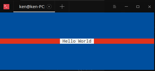
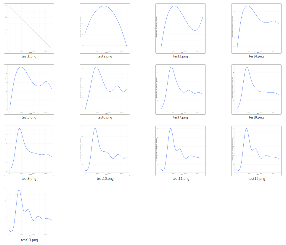
Let’s see an example of the plot.

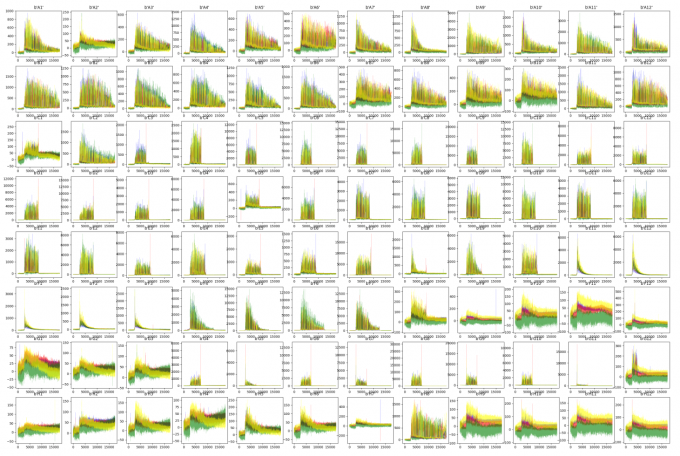
Familiar with Your Data

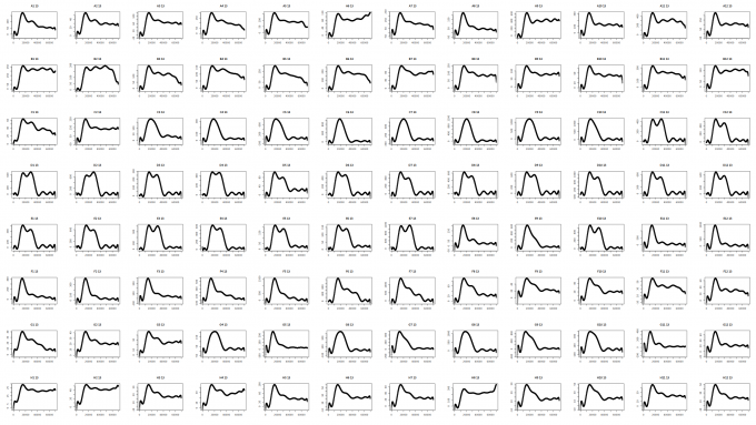
As we can see the result below, we have few types of pattern judged by the naked eyes:

• A01: Triangle. (The signal is decreasing but is still readable)
• A02: Flat. (Which doesn’t have signal at all)
• A08: Laying-Trapezoid. (The perfect result we’d love to)
• F01~F07: Acute Triangle. (Which means the signal is decreasing and the result is unreadable)
• C02: Stick. (Short sequence or Signal-Break due to some reasons.)

Though, it is easy to acquire a model from ML by putting all those check-point into a matrix and training them. But I decided to reduce the burden of my computer.

By first, I’d like to try something like linear regression.

Linear Regression

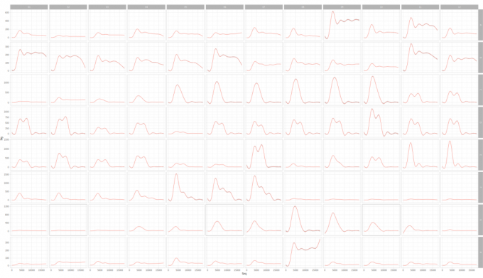
First, Let’s take a quick look of the smooth line

Now, let’s try the linear regression.
Main codes can be found at my blog

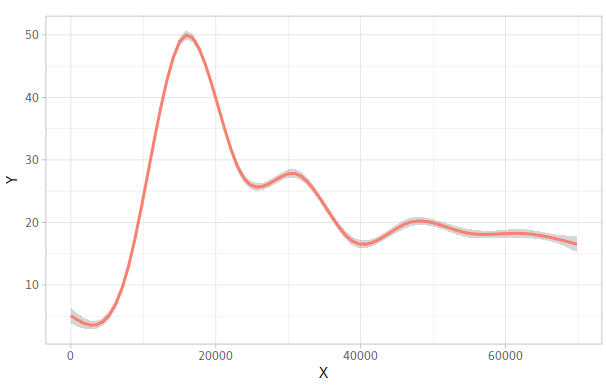
Let’s take the well H12 as an example
By using geom_smooth from ggplot2, we can achieve these graphics easily.

By calculating the regression function by lm with the exponent from 1 to 13, we can get the result as below

An example of regression function:

$$
f(x)= -5.33506521414874 e^{-56} * x^{13}+2.33068989275763 e^{-50} * x^{12}
$$

$$
-4.44202743547308 e^{-45} * x^{11}+4.8269078976017 e^{-40} * x^{10}
$$

$$
-3.27011035492282 e^{-35} * x^9+1.40852725678933 e^{-30} * x^8
$$

$$
-3.68400537011035 e^{-26} * x^7+4.64218496851634 e^{-22} * x^6
$$

$$
+2.12911181720032 e^{-18} * x^5-1.64587230405762 e^{-13} * x^4
$$

$$
+2.2678114895877 e^{-09} * x^3-1.27776012720345 e^{-05} * x^2
$$

$$
+0.0270106008326289 * x^1 -8.24054735022609
$$

As we can see, the last diagram is almost about the same as the result of geom_smooth!

Another awesome thing is it takes only a second to get the result!!

As we can see, the function of linear-regression is enough to tell us about that this well is failed or succeed and we can use the numbers from it to train our model!

Let’s check all the regression plot

It looks well, but it takes long time to make.

Click to see hidden codes

library(sangerseqR)
library(reshape2)

mylr = function(x,y){
  x_mean = mean(x)
  y_mean = mean(y)
  xy_mean = mean(x*y)
  xx_mean = mean(x*x)
  yy_mean = mean(y*y)

  m = (x_mean*y_mean - xy_mean)/(x_mean^2 - xx_mean)
  b = y_mean - m*x_mean

  f = m*x+b# 线性回归方程
  sst = sum((y-y_mean)^2)
  sse = sum((y-f)^2)
  ssr = sum((f-y_mean)^2)
  result = c(m,b,sst,sse,ssr)
  names(result) = c('m','b','sst','sse','ssr')
  result['ssr']/result['sst']
}

F_equation <- function(X,Formula){
  eval(parse(text = Formula))
}

LMEE <- function(TB,Times){
  colnames(TB)=c("X","Y")

  Group_X = "X"
  for(i in c(2:Times)){
    X_i = paste("I(X^",i,")",sep="")
    Group_X = paste(Group_X,X_i,sep=" + ")
  }
  str_lm = paste("lm(Y ~",Group_X, ', data=TB)', sep=' ')
  model = eval(parse(text = str_lm))

  Formula = model$coefficients[1]
  for(i in c(Times:1)){
    X_tmp = paste(model$coefficients[i+1], " * X^", i, sep="")
    Formula = paste(Formula,X_tmp,sep="+")
  }

  R2 = mylr(TB$Y,F_equation(TB$X,Formula))

  result = c()
  result$R2 = R2[[1]]
  result$model = model
  result$Formula=Formula

  return(result)
}

MEES <- function(TB, Times){
  colnames(TB)=c("X","Y")
  for(i in c(1:Times)){
    Result = c()
    if(i == 1){
      model <- lm(formula = Y ~ X, data = TB)
      Formula = paste(model$coefficients[1]," + ", model$coefficients[2]," * X", sep="")
      R2 = mylr(TB$Y,F_equation(TB$X,Formula))
      Result_TB = data.frame(Exp=i,R2=R2, F = Formula)
    }
    else{
      Result_LMEE = LMEE(TB,i)
      Result_tmp = data.frame(Exp= i, R2= Result_LMEE$R2, F = Result_LMEE$Formula)
      Result_TB = rbind(Result_TB, Result_tmp)
    }
  }
  return(Result_TB)
}

MEES_plot <- function(TB,Result_TB,header="test"){
  MAIN = as.character(TB$tube[1])
  colnames(TB)=c("X","Y")
  Result_TB = na.omit(Result_TB)
  Exp = nrow(Result_TB)
  Result_TB = Result_TB[order(Result_TB$R2, decreasing = T)[1],]
  X = unique(as.integer(TB$X/100))*100
  plot(X, F_equation(X,as.character(Result_TB$F)),type='p',
  main = paste(MAIN, Exp),
  xlab = "",
  ylab = "" )
}

TB_get <- function(ab1){
  A <- read.abif(ab1)
  A_raw = A@data$DATA.1
  T_raw = A@data$DATA.2
  C_raw = A@data$DATA.3
  G_raw = A@data$DATA.4
  tmp <- melt(t(data.frame(A_raw,T_raw,C_raw, G_raw)))
  return(list(tmp, A@data$TUBE.1))
}

png('../test.png',w=1920*1.3,h=1080*1.3)
par(mfrow=c(8,12))
for(i in dir()){
  print(i)
  TB_tmp = TB_get(i)[[1]]
  TUBE = TB_get(i)[[2]]
  TB = data.frame(X=c(1:nrow(TB_tmp)),Y=TB_tmp$value, tube=TUBE)
  MEES_plot(TB,MEES(TB,20))
}
dev.off()

Logarithmic Regression

$$
f(x) = log(x)+B
$$

Click to see hidden codes

library(sangerseqR)
library(reshape2)

mylr = function(x,y){
  x_mean = mean(x)
  y_mean = mean(y)
  xy_mean = mean(x*y)
  xx_mean = mean(x*x)
  yy_mean = mean(y*y)

  m = (x_mean*y_mean - xy_mean)/(x_mean^2 - xx_mean)
  b = y_mean - m*x_mean

  f = m*x+b# 线性回归方程
  sst = sum((y-y_mean)^2)
  sse = sum((y-f)^2)
  ssr = sum((f-y_mean)^2)
  result = c(m,b,sst,sse,ssr)
  names(result) = c('m','b','sst','sse','ssr')
  result['ssr']/result['sst']
}

TB_get <- function(ab1){
  A <- read.abif(ab1)
  A_raw = A@data$DATA.1
  T_raw = A@data$DATA.2
  C_raw = A@data$DATA.3
  G_raw = A@data$DATA.4
  tmp <- melt(t(data.frame(A_raw,T_raw,C_raw, G_raw)))
  return(list(tmp, A@data$TUBE.1))
}

Result = c()
for(i in dir()){  
  A <- TB_get(i)
  Y = A[[1]]$value[-c(1:12000)]
  TB <- data.frame(X=c(1: length(Y)), Y = Y)
  Model <- lm(formula = Y ~ log(X), data = TB)
  Cur <- Model$coefficients[[2]]
  R2 <- mylr(TB$Y, Model$coefficients[[1]] + Model$coefficients[[2]]*log(TB$X))
  #print(paste(Cur, R2))
  Result <- c(Result, Cur,R2)
}
Result <- data.frame(matrix(Result, ncol = 2 , byrow = T))
Di = rep(0,96)
Di[Result$X1< -10] = 1
Di[Result$X2 < 0.1] = 0
pheatmap::pheatmap(matrix(Di, ncol = 12, byrow = T), cluster_rows = F, cluster_cols = F)
#

png('../test2.png',w=1920*1.3,h=1080*1.3)
par(mfrow=c(8,12))
Result <-c()
for(i in dir()){
  print(i)
  A <- read.abif(i)
  A_raw = A@data$DATA.1
  T_raw = A@data$DATA.2
  C_raw = A@data$DATA.3
  G_raw = A@data$DATA.4
  tmp <- melt(t(data.frame(A_raw,T_raw,C_raw, G_raw)))
  Num =100
  Y = apply(matrix(tmp$value, ncol=4*Num, byrow = T),1,max)
  X = c(1:length(apply(matrix(tmp$value, ncol=4*Num, byrow = T),1,max)))
  TB = data.frame(X=X,Y=Y)
  Model <- lm(formula = Y ~ log(X), data = TB)
  Cur <- Model$coefficients[[2]]
  R2 <- mylr(TB$Y, Model$coefficients[[1]] + Model$coefficients[[2]]*log(TB$X))
  #print(paste(Cur, R2))
  Result <- c(Result, Cur,R2)
  plot(X,Y)
}
dev.off()
Result <- data.frame(matrix(Result, ncol = 2 , byrow = T))

Di = rep(1,96)
Di[Result$X1> -10] = 0
Di[Result$X2 < 0.1] = 0
pheatmap::pheatmap(matrix(Di, ncol = 12, byrow = T), cluster_rows = F, cluster_cols = F)

Though, judging the result by Regression model is an appropriate way, but this algorithm seems preferring the raw data list.

I was tried to use 0 and 1 to replace the result of failed and success and running:

xgboost(data = dtrain, max.depth = 2, eta = 1, nthread = 2, nrounds = 2, objective = "binary:logistic")

It works. Not perfect, but acceptable.

Because I was trying to find a way to call bases from the raw abi file and failed, I using the Sequencing Analyzing software to made a post processing to get the sequence and quality grades of the bases. Once we have the quality matrix, we can have a better way to grade the result. My choice is calculating the mean value of the base-quality from 80 to 120 for several reasons:

• 120 base is enough to value a successful task.
• first 80 bases have low quality and usually was tossed.
• I’d like to collect the result though it’s a derogation-signal.

I choose R to achieve this because package sangerseqR can turn the quality grades to integer from bin16 format. And I don’t know how to achieve this in Python.

Read_abiDirector <- function(abi_director){
  # Reading List
  abi_list = dir(abi_director)
  # Initialize Result
  TB <- data.frame()
  # Start flower
  for(abi_file in abi_list){
    Plate = strsplit(abi_director,'/')[[1]][3]
    Well = strsplit(abi_file,'[.]')[[1]][1]
    abi_file = paste(abi_director,abi_file,sep="/")
    abi <- read.abif(abi_file)
    tmp <- data.frame(mean(abi@data$PCON.1[80:120]), Plate = Plate, Well = Well)
    tmp[[1]] <- tmp[[1]]/61*100
    print(tmp)
    colnames(tmp) <- "Mean"
    TB <- rbind(TB,tmp)
  }
  TB[[1]][is.na(TB[[1]])] = 0
  return(TB)
}

Once We had the label file, we can extract the matrix one by one and turn them to xgb.matrix to train our model.
here, I removed the objective = "binary:logistic" parameter, and increased the depths and rounds to 5.

xgboost(data = dtrain, max.depth = 2, eta = 1, nthread = 2, nrounds = 2)

I combined 16 plates which means it has 1536 samples to compact the training data set.
Though, 5 rounds is not enough (fails ratio > 4%), I don’t want the model be over fitted.
Since the training data is better than before, I get the best performance for ever.