Introduction of Bioinformatics

Introduction of Bioinformatics

Data units:

© Quora

5V of Big Data

• Volume
• Velocity
• Variety
• Veracity
• Value

Difinition of Bioinformatic

Bioinformatics is the use of computer databases and computer algorithms to analyze proteins, genes, and the complete collection of deoxyribonucleic acid (DNA) that comprises an organism (the genome).
– Bioinformatics and Functional Genomics (BFG) Book, 3rd Edition (2015):

Bioinformatics refers to “research, development, or application of computational tools and approaches for expand- ing the use of biological, medical, behavioral, or health data, including those to acquire, store, organize, analyze, or visualize such data.”
– National Institutes of Health (NIH)

GeneCards.org (Human)
Genome.ucsc.edu (Genome browser)

For tolls for this classes

• HUGO gene names

• Uniport

• RCSB protein structure databases (PDB)

• Human protein Atlas

• cBioPortal for cancer genomics

  • Frequency of the gene mutated in cancers

• Immune epotope database

  • Antibody Antigen

• Homolog

• Analog: Convergent evelution

Structure Alignment

Sequence Alignment

ClsutalW
Muscle
TCoffee

Markov Models for Multisequence Alignment

Wiki: Hiddne Markov Model

Profile Hiden Markove Models are simoly a way to represent the features of these aligned sequences from the same family using a statistic model.

Parts of the protein is important to this specific family.
HMMs can make a profile to each protein family.
We can take this profile for familiy specific and align the same protein family.

PS: The HMMs could build profiles for families. We can using the profile of the pritein family and align our sequence. So we can have a better weighted alignment result by the families feature implied in HMMs profils (pre-bild model)

Markove Chains: Sequences of random varibales in which the futrue variable is detemined by the present variable stochasitic/probabilistic process.

• First Order Markov model: the current event only depends on the immediatetly preceding event.
  Second order models uss the two preceding evetns,
  THird order models use three, etc.

s

Learn all the insert and the deleted probabilistic from the aligned sequence database and build the model. Then we can evaluate the this family of the

Aligned Sequence for build the Markove Model

• Who do we get a proprate aligned sequence?
• What is the golden standard of the apropriate aligned squence?

How to buidl

• Remvove low occupancy columns (> 50%)

• Assign match states, delete states, insert states from MSA

• Get the path of each sequence

• Count the amino acid freqencies emitted from match or insert states, which are converted into probabilities for each state

• Count…

• Tran model using a given multiple sequence alignment

  • Baum-Welch Algorithm odes the training/parameter estmation for HMM
  • Baum-Welch is an ecpetation-Maximization (EM) algorithm - iterative
  • Converges on a set of probabilities for the model that best fir the multiple alignment you gaie it
  • Only finds a local maxima - good to try different intial conditions
  • Baum-Welch can also perfom an MSA to from a set of unaligned sequences

• faster and more fitable than PIS-blast

• Classification: wihch fimaily of protein belongs.

Meloular Phyligenies

Describ, Meaning, Access Confidence.

NGS

Sanger Sequencing

reciprocal translocation: long reads align

© C.V.Beechey A.G.Searle

Genome Sequencing

Sequencing and Diseases

Sample workflow

DNA → Library → capture based selection → Sequencing
DNA → PCR based selection→ Library → Sequencing

Exp

Severe combined immunodeficiency syndrome

Il-2/4/7/9/15/21 → X-SCID (γ domain)

γ domain mutate failed to active jak3 → Jak3-SCID

Newborn sscreening

• Amino acid disorder
  • PKU; MSUD
• Fatty acid disorder
  • MCAD; VLCAD
• Organic acid disorders
  • pH disorder

Card screen

• Hemoglobinopathies
  • Sickle cell, SC, S-β-thalassemia
  • MSUD
• Galactosemia
• CF; CF links
• SCID - recommended by HRSA, detects T cell receptro excision circles (TRECs)
  • T cell recombination.

TREC screening

• False positive
• False negatives
  • Zap70 deficiency
  • MHC Class II deficiency
  • NF-κb essential modulator
  • late-onset ADA
• Positive: Genes tsted: ADA CD3D; CD3E…
  FOXN1: required for the development of Thymus
  • WES, WGS
    • Can detect novel variants
    • Often uses trios or unaffected sibs
    • Can be used in CMC-STAT3 gof, IL-17R mutations

CF Screening -immunoreactive trypsinogen

• Typically measured by fluoroimmunoassay
• False postive
  • Perinatal asphyxia, infection
  • CF carrier (heterozygote)
• False negatives - rare
  • Lab or specimen error
  • pseudo-Bartter’s syndrome
    Positive:
• Sweat test
  • high salting in sweat; less salting concentration among patients
  • dehydrate
• Genetic testing

Bordeline sweat test

• Targeted sequence of CFTR

Challenges of WGS, WES

• Each individual harbors 2.7-4.2m SNV

NGS and cancer

• Can compare somatic to germline mutation
  • Exmaple AML
  • Micro-dissected tumor
  • Circulating tumor RNA

Cancer Early Casses

• Lukas Whartman

  • Dx All 2003

  • Treatede with sibling related …

  • Sequenced the cancer genome for actionable mutations

  • No mutations detected

  • RNAseq found iverexpression in FLT3

  • Remitted with FLT3 inhibitor(Sutent)

• 2nd stem cell transplatnt after remission
• Suffers from GVHD

Panels

• Sequences regions of interest

• Hybridization or PCR based

• Often disease specific

• Eg Breast , lung, colon CA

• Sequence coverage is high (up to 80x)

• GeneDx Panel data -positive yield

• 9.7% for breast

• 13.4% for ovarian

• 14.8% for colon/stomacj

• pathogenic or likely pathogenic mutation in over 8%-15% ofr …

• Between 70%-92% of the patients remains mutation-negative or undiagnosed
  …

• Mutations in PALB2 and ATM in pancreatic CA

• XRCC2, FANCC and BLM in HBOC

• Germline RNA-splice mutations using RNA-seq

• Germline splice variants in BRCA1/BRCA2

• …

• NF1

NGS and cancer - Clinical utility

• Diagnosis

• Survival prediction

  • GNAS & KRAS

• Up to 20% of NGS tests were actionable

• Another 50% were actionable if you include mutations that could be targeted by the use of a FDA approved drug for off-label use

• Can identify candidates for anti-EGFR therapies

• Re-classification of tumors.

  • Troditional: look unde the microscopy

Pathology

• Diagnosis
  • Useful in small smaples -FNAs
  • Thyroseq panel for thyroid cancer
• Survival prediction

Liquid Biopsy

• Rationable
  -Has been used for liquid and solid tumors
• May be useful in lieu of biospy…

Pharmacogenomics

• Ratoionale
• Exampel
  • Dihydropyrimidine dehydrogenase:D{D
  • Mutations associated with greate toxicity of 5-fluorouracil, capecitiabine and…

Futrue Directions for CA

• Epigenome
  • CHIP-seq (Bulk cell)
  • ATAC-seq (More advance; nano scale cells.)
    -RANseq
  • Transcriptomes including non-coding RNA

- -

TPM: normalized by the size of the library

• Different tissues has different expression profile and the size of the profile is different.
• Transcripts is different, too.

Small RNA

1. Non coding RNA
2. Long non-codong RNAs
3. siRAN, piRNA, snRAN, snoRNAs
4. biogenesis and functions of miRNA
5. qRT-PCR, Microarrary Deep Sequencing
6. structure features of snRANs and snoRNAs
7. role of miRNAs ine cancer
8. IncRNA XIST in X chrmosome

Coding RNAs vs Non-coding RNAs

Major type of small RNA

• tRAN
• Ribosomal RNA
• Smal neclear RNA (snRNA)
• Small nucleolar RNAs (snoRNAs)
• MicroRNAs (miRNAs)
• Small interfering RNAs (siRNAs)
• Piwi-interacting RNAs (piRNAs)

Long

• 18/28S rRNAs
• Long intergenic non-coding rNASs or long intronic non-coding RANS
• Telomere-associated lncRNAS

Long non-coding RNA

• > 200nt
• 56,018 and 46,475 of long non coding RNA genes for human and mouse
• LncRNAs represent the largest category of ncRNAs
• XIST and H19 represetn the most extensicely studied lncRNAs
• X-inactive-specific trancripts (XIST): inactivation inactive X chromosome

.

---

miRNA: Perfect complemetnatrity/Non-perfect complemetnatrity
piRNA: Silencing of trasnposable elements in the germline
siRNA: Perfect match

Evolutionary caonservation of has-miR-140-5p

This miRNA is concertive amone vertibirets. (Human; Orangutan; zabera fish)

1993: C-elegans
2002: Biomarker; First version of the miRNA DB (V1)
2004: miRNA Microarray; RNAhybrid; V3,4,5
2006: miRNA-Seq; TarBase(MC) V8,9

Tools

Dyana Scan; d

Cluster

What is cluster

A cluster refers to “a group that includes objects with similar attributes” (e.g., Pirim et al., 2012)

• (1) a set of data objects that are similar to each other, while data objects in different clusters are different from one another
• (2) a set of data objects such that the distance between an object in a cluster and the centroid of the cluster is less than the distance between this object to centroids of any other clusters
• (3) a set of data objects such that the distance between any two objects in a cluster is less than the distance between any object in the cluster and any object not in it
• (4) a continuous region of data objects with a relatively high density, which is separated from other such dense regions by low-density regions

Object:
Finding groups of data objects such that those data objects grouped in the same cluster will be similar (or related) to one another, and different from (or unrelated to) the data objects grouped in the other clusters

Exp:

© Gergely Tholt, et al, 2018

How Clustering is Different from Classification

• Clustering does not use a subset of data objects with known class labels (called “train set”, which is commonly used in classification) to learn a classification model (i.e., “supervised learning”)

• Clustering is deemed as a form of an unsupervised task, which computes similarities (based on a distance) between data objects, without having any information on their correct distributions (also known as ground truth)

• Due to its unsupervised nature, clustering is known to be one of the most challenging tasks. The different clustering algorithms developed during the years by the researchers, lead to different clusters to the same dataset, even for the same algorithm, the selection of different parameters or the presentation order of data objects may greatly affect the eventual clustering partitions

How it works

1. Confirm data is metric
2. Scale the data
3. Select Segmentation Variables
4. Define similarity measure
5. Visualize Pair-wise Distances
6. Method and Number of Segments
7. Profile and interpret the segments
8. Robustness Analysis
   Cite: T. Evgeniou^[1]

Major Types of Clustering Algorithms

© Adil Fahad; 2014

Commonly Used Types of Clustering Algorithms in Biomedical Research

The 3 commonly used types of clustering algorithms are:

• Hierarchical-based clustering considers grouping data objects with a sequence of nested partitions, and attempts to build a tree-like, nested, hierarchical structure that partitions a dataset
• Partitioning-based clustering partitions a dataset into a particular # of clusters denoted by K, no hierarchical structure, and therefore attempts to seek a K-partition of a dataset
• Model-based clustering [e.g., mclust, Expectation-Maximization (EM), COBWEB, and Self-Organizing Map (SOM)] applies predefined mathematical models for fitting the dataset and then, tries to optimizes them. The basic assumption is that the dataset is a mixture (i.e., hybrid) of several probability distributions. Such algorithms can determine the # of clusters based on standard statistical approaches (e.g., maximum likelihood), which could be robust to outliers and noise

These commonly used types of clustering algorithms serve well to fulfill the objective of biomedical research to extract knowledge from big data, and their applications in biomedical research are ubiquitous in the prevention, treatment, and prognosis of human diseases!

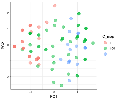
Partitioning

library klaR

library(klaR)
library(ggplot2)
library(reshape2)
library(psych)


set.seed(1)
x <- rbind(matrix(rbinom(250, 2, 0.25), ncol = 5),
           matrix(rbinom(250, 2, 0.75), ncol = 5))
colnames(x) <- c("a", "b", "c", "d", "e")

## run algorithm on x:
cl <- kmodes(x, 2)
cl2 <- kmeans(x, 2)

# plot the result

x <- data.frame(x)
PC <- principal(x[1:5], nfactors=2, rotate ="none")
pc <- data.frame(PC$scores)

C_map <- cl$cluster
C_map[which(cl$cluster!= cl2$cluster)] =100
C_map <- as.character(C_map)

ggplot(pc, aes(x=PC1, y=PC2, color = C_map)) +
  geom_point(size=4,alpha=0.5)+ theme_bw()

The color blue is the different results from two clusters. As we can see here, it doesn’t matter which group they blong since they are on the intersect region of two group.

But when the K-mean increase to 3, they had a good agreement on group 1 and 3, but have misaggrement on group 2.

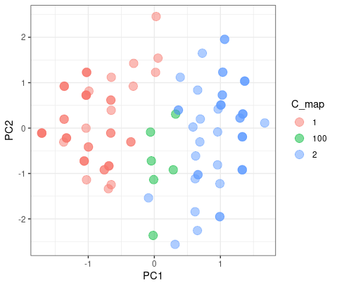© Karobben; 2022

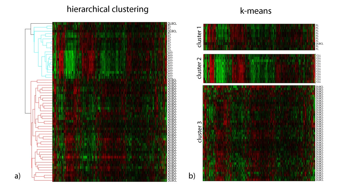
Hierarchical Clustering Algorithms

Hierarchical clusters are built on a cluster hierarchy also known as a tree of clusters called a dendrogram. These algorithms allow us to explore the dataset at different granularity levels, which are also called connectivity-based algorithms that build clusters gradually.

• Agglomerative hierarchical clustering, also called bottom-up approach, starts from bottom with each data object placed individually in a separate group (i.e., n clusters). Then, it successively merges data objects or groups that are close to (i.e., similar to) one another. This repeats till all the groups are eventually merged into a single hierarchical cluster, which is the topmost level of the hierarchical tree. This merging process will continue until a certain stopping condition is valid
• Divisive hierarchical clustering, also called as top-down approach, begins from topmost level by placing all data objects in a single cluster, and every successive iteration will split a cluster into smaller clusters (i.e., subsets). This dividing process happens until eventually each data object is placed as a single cluster (i.e., n clusters at the bottommost level), or a certain stopping condition is valid

Distance Measures (also called Dissimilairty Measures) in Hierarchical Clustering

© Rui Xu, et al. 2010

Major Linkage Methods of Agglomerative Hierarchical Clustering

• Single Linkage (also called Minimum Linkage)
• Complete Linkage (also called Maximum Linkage)
• Average Linkage [also called Unweighted Pair Group Method with Arithmetic Mean (UPGMA)]
• Centroid Linkage [also called Unweighted Pair Group Method with Centroid (UPGMC)]
• Ward’s Linkage (also called Minimum Variance)
• McQuitty Linkage [also called Weighted Pair Group Method with Arithmetic Mean (WPGMA)]

© Shaik Irfana Sultana; 2020[2]

Advantages and Disadvantages of Agglomerative Hierarchical Clustering and Divisive Hierarchical Clustering

• Agglomerative hierarchical clustering (A “bottom-up” approach) starts with n clusters, each of which includes exactly one data object. By comparison, divisive hierarchical clustering would start with considering 2(n-1) - 1 possible two-subset divisions for a cluster (a dataset) with data objects, which is very computationally intensive. Therefore, Agglomerative hierarchical clustering is a often preferred and more widely used approach

• Divisive hierarchical clustering (A “top-down” approach) provides clearer insights into the main structure of a dataset, because the larger clusters are generated at the early stage of the clustering process, and are less likely to suffer from the accumulated erroneous decisions, which can not be corrected by the successive process

• Advantages

  • They provide embedded flexibility regarding the level of granularity
  • It is easier for them to handle a variety of distance measures
  • They are applicable to any attribute types

• Disadvantages

  • The stopping criteria can be very vague to determine (i.e., the # of clusters can be difficult to determine)
  • Many hierarchical algorithms do not revisit the intermediate clusters once constructed, which hampers the purpose of their improvement

PS: after calss challenges

İzzet Tunç; 2021. Time serious data Clustring
tslearn; Time Series Clusterin
paper:NbClust: An R Package for Determining the Relevant Number of Clusters in a Data Set

NbClust package provides 30 indices for determining the number of clusters and proposes to user the best clustering scheme from the different results obtained by varying all combinations of number of clusters, distance measures, and clustering methods.

L10

NbClust: NbClust Package for determining the best number of clusters

L11

Partitional clustering

• Partitional clustering (also called partitioning-based clustering) algorithms identify the best K centers to partition the data objects into K clusters where the centers are either centroids (means), called K-means, or medoids, called K- medoids
• In contrast to hierarchical clustering, which yields a successive level of clusters by conducting either fusions or divisions, partitional clustering assigns a set of data objects into clusters with no hierarchical structure.
• The # of clusters, i.e., K, needs to be prespecified, and the choice of K is usually influenced by either prior knowledge regarding the nature of the data, or by using clustering validity measures.
• The K-means clustering algorithm is the best-known squared error-based clustering algorithm that has led to its applications in a variety of fields, e.g., psychology, marketing research, biology, and medicine

K-Means Clustering

• First proposed by Steinhaus (1956) [Others suggest Forgy (1965)] [Steinhaus H. Sur la division des corp materiels en parties. Bull Acad Polon Sci. 1956; IV (C1.III), 801-804 has been cited 1,312 as of 02/22/2022, according to Google scholar; Forgy EW. Cluster analysis of multivariate data: efficiency versus interpretability of classifications. Biometrics 1965;21:768-9 has been cited 2,991 as of 02/22/2022, according to Google scholar]

• The K-means algorithm (also called kmeans algorithm) finds the centroids (i.e., centers) to minimize the sum of the squares of the Euclidean distance between each data point (i.e., each data object) and its closest centroid (i.e., center)

• In general, the K-means iterative clustering method is implemented as follows:

  • Step 1: Choose a K value. Based on this value, randomly choose an initial set of K centroids
  • Step 2: Assign each data object to the cluster with the nearest centroid
  • Step 3: Determine the new set of K centroids for the K clusters, by computing the mean value of the cluster members - Step 4: Repeat Steps 2 and 3 until there is no change in the criterion function (i.e., sum of squared error function) after an iteration (i.e., the algorithm converges)

• The K-means algorithm is relatively scalable and efficient for processing (i.e., clustering) large datasets. However, K-means can converge to a local optimum (rather than a global optimum) in a small # of iterations

Iteration

K-means clustering is a good place to start exploring an unlabeled dataset. The K in K-Means denotes the number of clusters. This algorithm is bound to converge to a solution after some iterations. It has 4 basic steps:

1. Initialize Cluster Centroids (Choose those 3 books to start with)
2. Assign datapoints to Clusters (Place remaining the books one by one)
3. Update Cluster centroids (Start over with 3 different books)
4. Repeat step 2–3 until the stopping condition is met.

You don’t have to start with 3 clusters initially, but 2–3 is generally a good place to start, and update later on.
© Azika Amelia; 2018; K-Means Clustering: From A to Z

© Azika Amelia; 2018

Limitation

It is sensitive to the densities, the size of the cluster.

Advantages

1. Is simple and can be easily implemented in solving many practical problems
2. Can work very well for compact and hyperspherical clusters
3. Can be used to cluster large datasets

Disadvantages

1. There is no efficient and universal method for identifying the initial partitions and the # of clusters, i.e., K. The convergence centroids vary with different initial points. A general strategy for the problem is to run the algorithm several times with random initial partitions
2. The iterative optimization procedure of K-means cannot guarantee convergence to a global optimum. The stochastic optimization techniques, e.g., simulated annealing (SA) and genetic algorithm (GA) can find the global optimum, but these tehniques are computationally intensive
3. The K-means is sensitive to outliers and noise. E.g., even if a particular data object is quite far away from the cluster centroid, it is grouped into a cluster and, thus, could distort the cluster’s shape
4. The definition of means limits the application only to numerical variables

Example of the K-means cluster

© Marcilio CP de Souto, et al.

Advantages and Disadvantages of PAM Clustering

Advantages

1. PAM is more general than K-means [that typically require attributes (i.e., features) to be continuous], which can handle all types of attributes and all types of distance metrics (i.e., distance measures)
2. Medoids (rather than centroids) are applied as the cluster “centers”, which are more robust and less sensitive to outliers and noise
3. PAM can assist a user to determine the optimal # of clusters, i.e., K, because it provides a silhouette plot showing the silhouette widths for the K clusters

Disadvantages

1. The # of clusters, i.e., K, needs to be pre-specified, and the eventual clustering results are dependent on the initial selection of a random set of K data objects as K medoids
2. The iterative optimization procedure of PAM cannot guarantee convergence to a global optimum
3. PAM could be computationally intensive, which could work effectively for small datasets, but does not scale well for large datasets. To handle large datasets, a sampling-based method, called CLARA (Clustering LARge Applications), can be applied

t-SNE

t-distributed Stochastic Neighbor Embedding

• The t-distributed Stochastic Neighbor Embedding (t-SNE) (van der Maaten, 2008) is a state-of-the-art nonlinear dimensionality reduction algorithm, that has emerged as a popular and powerful technique for the analysis of single-cell data generated by a wide variety of experimental platforms (e.g., Camp et al., 2017; See et al., 2017; Lavin et al., 2017)
• The t-SNE focuses on preserving the local structure while de-emphasizing the global structure of high-dimensional data, resulting in similar data points clustering together in an unsupervised manner. Because t-SNE allows the user to define the # of dimensions for analysis, cell populations can be unbiasedly shown in 2 or 3 dimensions
• For a high-dimensional dataset, t-SNE creates a low-dimensional distribution, or a ‘map’. Conspicuous groupings of data points, also called ‘islands’, correspond to observations that are similar in the original high-dimensional space, which help to visualize the general structure and heterogeneity of a dataset

Exp:

© Paul A. Reyfman, etl al.

Code in R

# Data simulation

set.seed(627)
Bluegill.length <- sample(seq(15, 22.5, by=0.5), 50, replace=T)
Bluegill.weight <- sample(seq(0.2, 0.8, by=0.05), 50, replace=T)
Bowfin.length <- sample(seq(46, 61, by=0.5), 50, replace=T)
Bowfin.weight <- sample(seq(1.36, 3.2, by=0.5), 50, replace=T)
Carp.length <- sample(seq(30, 75, by=1), 50, replace=T)
Carp.weight <- sample(seq(0.2, 3.5, by=0.1), 50, replace=T)
Goldeye.length <- sample(seq(25, 38, by=0.5), 50, replace=T)
Goldeye.weight <- sample(seq(0.4, 0.54, by=0.01), 50, replace=T)
Largemouth_Bass.length <- sample(seq(22, 55, by=0.5), 50, replace=T)
Largemouth_Bass.weight <- sample(seq(0.68, 1.8, by=0.01), 50, replace=T)

weight <-c(Bluegill.weight, Bowfin.weight, Carp.weight, Goldeye.weight,
Largemouth_Bass.weight)
length <-c(Bluegill.length, Bowfin.length, Carp.length, Goldeye.length,
Largemouth_Bass.length)

set.seed(627)
speed <- rnorm(50*5, 7.2, sd=1.8)
fish <- c(rep("Bluegill", 50), rep("Bowfin", 50), rep("Carp", 50),
rep("Goldeye", 50), rep("Largemouth_Bass", 50))
fish.data <- data.frame(length, weight, speed, fish)
str(fish.data)


# K-means clustering
# Apply kmeans() function to perform K-means clustering
# Apply the set.seed() function to make the results of kmeans() function repeatable
set.seed(627) # the random for the random start of the centroid
fish_data_kmeans <- kmeans(fish.data[,1:3], centers = 5, nstart=1)
str(fish_data_kmeans)
fish.data$cluster <- as.factor(fish_data_kmeans$cluster)
# The following R code is equivalent to table(fish.data$cluster, fish.data$fish)
with(fish.data, table(cluster, fish))

  cluster Bluegill Bowfin Carp Goldeye Largemouth_Bass
        1       50      0    0       3               4
        2        0      7   17       0               0
        3        0      0   13      47              18
        4        0     13   14       0              21
        5        0     30    6       0               7

# Compute clustering accuracy
cluster_fish <- as.matrix(table(fish.data$cluster, fish.data$fish))
cluster_fish
sum(diag(cluster_fish))/sum(cluster_fish)
# [1] 0.308

# Partitioning Around Medoids (PAM) clustering
library(cluster)
set.seed(627)
fish.data_pam <- pam(fish.data[,1:3], k=5)
str(fish.data_pam)

fish.data_pam$clustering[1:10]
fish.data_pam$clustering[241:250]

# Create a 1x2 grid for plotting
par(mfrow=c(1,2))
# Create a graphical display of PAM clusters and a silhouette plot by applying plot() function
plot(fish.data_pam, main="PAM")

# Reset to a 1x1 grid for plotting
par(mfrow=c(1,1))

fish.data$pam_cluster <- as.factor(fish.data_pam$clustering)



# The following R code is equivalent to table(fish.data$pam_cluster, fish.data$fish)
with(fish.data, table(pam_cluster, fish))

# Compute clustering accuracy
pam_cluster_fish <- as.matrix(table(fish.data$pam_cluster, fish.data$fish))
pam_cluster_fish

sum(diag(pam_cluster_fish))/sum(pam_cluster_fish)
# [1] 0.536



# t-Distributed Stochastic Neighbor Embedding (t-SNE) Clustering

# R code for t-SNE clustering

#setwd("C:\\Users\\Tianhua Niu\\Desktop")
#data_tsne <- read.delim("data_1.txt", header = T, stringsAsFactors = F, sep = "\t")
str(data_tsne)

library(caret)
library(Rtsne)

# Apply the set.seed() function to make the results of Rtsne() function repeatable
set.seed(627)
tsne_model_1 <- Rtsne(as.matrix(data_tsne), check_duplicates=FALSE, pca=TRUE, perplexity=30, theta=0.5, dims=2)

# Create a data frame based on tsne_model_1
d_tsne_1 <- as.data.frame(tsne_model_1$Y)
str(d_tsne_1)

library(ggplot2)
# Plotting the t-SNE result by applying ggplot() function
# plotting the results as a scatter plot without clustering
ggplot(d_tsne_1, aes(x=V1, y=V2)) +
  geom_point(size=0.25) +
  guides(colour=guide_legend(override.aes=list(size=6))) +
  xlab("tSNE_1") + ylab("tSNE_2") +
  ggtitle("A 2-Dimensional t-SNE Plot") +
  theme_light(base_size=12) +
  theme(axis.text.x=element_blank(),
        axis.text.y=element_blank(), plot.title = element_text(hjust = 0.5)) + scale_colour_brewer(palette = "Set2")

# Save the original dataset d_tsne_1 into a data frame called d_tsne_1_original
d_tsne_1_original <- d_tsne_1

# Create a hierarchical clustering model using complete linkage method, and save the output into an R object called fit_cluster_hclust
dist_euclid <- dist(scale(d_tsne_1), method = "euclidean")
fit_cluster_hclust <- hclust(dist_euclid, method = "complete")

# setting k=3 clusters as output for hierarchical clustering model
d_tsne_1_original$cl_hclust <- factor(cutree(fit_cluster_hclust, k=3))

# Create a K-Means clustering model, and save the output into an R object called fit_cluster_kmeans
# Apply kmeans() function to perform K-means clustering
# Apply the set.seed() function to make the results of kmeans() function repeatable
set.seed(627)
fit_cluster_kmeans <- kmeans(scale(d_tsne_1), centers = 3, nstart=1)
d_tsne_1_original$cl_kmeans <- factor(fit_cluster_kmeans$cluster)


# Create a plot_cluster() function
plot_cluster <- function(data, var_cluster, palette)
{
  ggplot(data, aes_string(x="V1", y="V2", color=var_cluster)) +
  geom_point(size=0.25) +
  guides(colour=guide_legend(override.aes=list(size=6))) +
  xlab("") + ylab("") +
  ggtitle("") +
  theme_light(base_size=12) +
  theme(axis.text.x=element_blank(),
        axis.text.y=element_blank(),
        legend.direction = "horizontal",
        legend.position = "bottom", legend.text = element_text(size = 12),
        legend.box = "horizontal") +
    scale_colour_brewer(palette = palette)
}

# Apply plot_cluster() function
plot_hclust <- plot_cluster(d_tsne_1_original, "cl_hclust", "Set1")
plot_kmeans <- plot_cluster(d_tsne_1_original, "cl_kmeans", "Accent")

# Put these 2 plots side by side by applying R package gridExtra
library(gridExtra)
grid.arrange(plot_hclust, plot_kmeans, ncol=2)

L16 Random Forest

© Jesse Johnson

Bagging: Bootstrap Aggregating

• Bagging algorithm, an ensemble learner, is a type of ensemble learning (also called committee- based learning) methods inspired from real life phenomena like democratic process, expert teams, and others, to combine individual machine learning methods into one predictive model in order to decrease the variance of the predictive model, and each individual machine learning method is called a base learner

• In Bagging algorithm, each base learner (i.e., individual learner) is constructed independently from a “bootstrap sample” (“bootstrap” refers to “resampling with replacement”) of the original train set, such that multiple base learners are trained by the same machine learning method on different base learner-specific train sets (i.e., different "bootstrap samples“). During iteration, the successive base learners do not depend on earlier base learners (i.e., all are built independently),. Eventually, either a majority voting of predictions (for classification) or an averaging of predictions (for regression) is taken. Therefore, the diversity of individual learners is emphasized in Bagging algorithm, which has been increased implicitly for this ensemble learner

Omics

---

1. Cluster Analysis and Segmentation ↩︎

2. Shaik Irfana Sultana, 2020, How the Hierarchical Clustering Algorithm Works; Dataaspirant ↩︎