SNP is fun: Tricks for dealing with VCF files

Extrack Fasta from VCF file

basic usage:
MatthewP, 2019: cat ref.fa | vcf-consensus your_file.vcf.gz > out.fa

bgzip -c file.vcf > file.vcf.gz
tabix -fp vcf file.vcf.gz
cat ref.fa | vcf-consensus file.vcf.gz > out.fa

Extrack Mitonchondira Genome Only

grep -E "mitochondrion_genome|#" ../VCF3/ActtsNICD18WDF_aln_pe_bqsr.bam.vcf > file.vcf
bgzip -c file.vcf > file.vcf.gz
tabix -fp vcf file.vcf.gz
cat ref.fa | vcf-consensus file.vcf.gz > out.fa

Check the highly mutated Genes

for line in {1..13};
do
    GENE=$(grep -i mitochondrion_genome  ../../Yuwei_data/DATA/genes.gtf | grep mRNA| awk 'NR=='$line'{print $12}')
    SL=$(grep -i mitochondrion_genome  ../../Yuwei_data/DATA/genes.gtf | grep mRNA| awk 'NR=='$line'{print $4}');
    SR=$(grep -i mitochondrion_genome  ../../Yuwei_data/DATA/genes.gtf | grep mRNA| awk 'NR=='$line'{print $5}')
    echo $GENE
    grep -i mitochon ../VCF3/* | awk '$2>='$SL''| awk '$2 <='$SR'' | awk -F: '{print $1}'| uniq -c| grep -iv h_
done

for loop

..
├── VCF3
└── VCF3_mt
    └── Mito.fa

vcf files are in VCF3, script is running in VCF3_mt. Mito.fa is the Reference

for i in $(ls ../VCF3/*);
    do file=$(echo $i|sed 's=../VCF3/==;s/_aln_pe_bqsr.bam.vcf//')
    grep -E "mitochondrion_genome|#" $i > $file.vcf
    bgzip -c $file.vcf > $file.vcf.gz
    tabix -fp vcf $file.vcf.gz
    cat Mito.fa|  vcf-consensus $file.vcf.gz > $file.fa
done

#rm -f  *vcf*

# Change the Names
for i in $(ls *.fa| grep -v Mito); do NAME=$(echo $i| sed 's/.fa//'); sed -i "s/>/>$NAME /" $i;done

cat *.fa > All.fa


# Quick Tree with ClustalW
clustalo -QUICKTREE -OUTPUT=FASTA  -INFILE=All.fa
clustalw -QUICKTREE -OUTPUT=FASTA  -INFILE=All.fasta -CLUSTERING=NJ -BOOTSTRAP=1000

library("ggtree")
tree <- read.tree("/run/user/1000/gvfs/sftp:host=129.81.246.249,user=ken/home/ken/Mutation/Raw_VCF/VCF3_mt/All.dnd")
ggplot(tree, aes(x, y)) + geom_tree() + theme_tree() + geom_tiplab(size=5, color="purple") +xlim(NA, 0.04)

Visualization

SNP ratiol change

1. Cat all vcf files into one
   grep -v "#" *.vcf| awk '{OFS="\t"; print $1,$2,$4,$5}' |sed 's/:/\t/' > All_vcf.csv

2. Visualization by ggplot

library(ggplot2)
library(stringr)
library(patchwork)

TB <- read.table("G3_all_vcf.csv")
colnames(TB) <- c("Sample", "Chrom", "Loc", "Ref", "Alt")
TB$SNP <- paste(TB$Ref, TB$Alt)

TB <- TB[TB$Ref %in% c("A", "G", "T", "C"),]
TB <- TB[TB$Alt %in% c("A", "G", "T", "C"),]

TB$SNP <-  str_replace_all(TB$SNP, "G T", "C A")
TB$SNP <-  str_replace_all(TB$SNP, "G A", "C T")
TB$SNP <-  str_replace_all(TB$SNP, "G C", "C G")
TB$SNP <-  str_replace_all(TB$SNP, "A G", "T C")
TB$SNP <-  str_replace_all(TB$SNP, "A T", "T A")
TB$SNP <-  str_replace_all(TB$SNP, "A C", "T G")

ggplot(TB, aes(Sample, fill= SNP)) + geom_bar(show.legend = F) + theme_bw()+ theme(axis.text.x = element_text(angle = 90,hjust = 1, vjust = .5))

TB2 <- cbind(TB,as.data.frame(str_split_fixed(TB$Sample, "_", 2)))
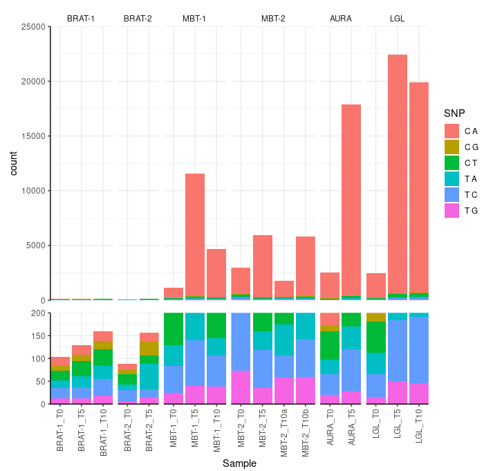
TB2$V1 <- factor(TB2$V1, levels =c("BRAT-1", "BRAT-2", "MBT-1", "MBT-2", "AURA", "LGL"))
TB2$Sample <- factor(TB2$Sample, levels =unique(TB2$Sample[order(TB2$V2)]))

P <- ggplot(TB2[TB2$V2!="Donor",], aes(Sample, fill= SNP)) + geom_bar() + theme_bw()+
   theme(axis.text.x = element_text(angle = 90,hjust = 1, vjust = .5)) + facet_grid( ~V1, space = 'free', scales = 'free')


P1 <- P + coord_cartesian(y=c(0, 25000), expand = F)  + theme(strip.background = element_blank(), axis.title.x = element_blank(), axis.text.x = element_blank(), axis.ticks.x = element_blank(), panel.border = element_blank(), axis.line.y.left = element_line())
P2 <- P + coord_cartesian(y=c(0, 200), expand = F)+ theme(strip.background = element_blank(), axis.title.y = element_blank(), strip.text = element_blank(), legend.position = "None", panel.border = element_blank(), axis.line.y.left = element_line(), axis.line.x.bottom = element_line())

GGlay = 'A
A
A
B
'
P1 +P2 +plot_layout(design = GGlay)

---