Gene Set Enrichment Analysis (GESA) in R

How it works and why it matters

Here is an example explained by ChatGPT

Suppose we have a gene expression dataset consisting of 6 genes (A, B, C, D, E, and F) and 3 samples (S1, S2, and S3), and we want to test whether a pre-defined gene set called “MySet” is enriched in this dataset. Here’s the dataset:

Gene	S1	S2	S3
A	1	2	1
B	2	4	1
C	3	6	2
D	4	8	3
E	1	2	1
F	2	4	1

The first step in GSEA is to rank the genes based on their correlation with the phenotype of interest. In this example, we will use the sum of expression values across samples as the phenotype. The ranked list of genes based on this phenotype is:

Gene	Rank
D	15
C	11
B	7
F	7
A	4
E	4

The second step is to calculate an enrichment score for the gene set “MySet” by walking down the ranked list of genes, and computing a running sum of the signed correlation between each gene and the phenotype. If a gene is in “MySet”, its correlation is positive; otherwise, it is negative. The enrichment score is the maximum deviation from zero of the running sum. Here’s the calculation:

Gene	Rank	In MySet?	Correlation	Running Sum
D	15	No	-1	-1
C	11	No	-1	-2
B	7	Yes	+1	-1
F	7	Yes	+1	0
A	4	Yes	+1	1
E	4	No	-1	0

The maximum deviation from zero of the running sum is 1, which occurs at gene A. Therefore, the enrichment score for “MySet” is 1.

This example demonstrates the basic steps of GSEA, but in practice, GSEA is often applied to much larger datasets and gene sets, and the significance of the enrichment score is assessed using statistical tests such as permutation tests or gene set permutation tests.

GESA

In clusterProfiler, there are functions designed to do GESA based on GO and KEGG gene sets. Here I am trying to show you how to do GESA with your customized data set.

There are two main functions which are GSEA from clusterProfiler and fgsea from fgsea. A quick enrichment analysis could be done by example data.

library(clusterProfiler)
library(plyr)
library(fgsea)

# loading example data set
data(examplePathways)
data(exampleRanks)

fgseaRes <- fgsea(examplePathways, exampleRanks, nperm=1000, maxSize=500, minSize = 10))

TERM2GENE = ldply(examplePathways, data.frame)
gse <- GSEA(gene = rev.default(exampleRanks) ,  TERM2GENE = TERM2GENE)
#gseaplot(gse, by = "all", title = gse$Description[1], geneSetID = 1)

Default Parameters for Two Functions

fgsea	GSEA
fgsea( pathways, stats, nperm, minSize = 1, maxSize = Inf, nproc = 0, gseaParam = 1, BPPARAM = NULL)	GSEA( geneList, exponent = 1, nPerm = 1000, minGSSize = 10, maxGSSize = 500, pvalueCutoff = 0.05, pAdjustMethod = "BH", TERM2GENE, TERM2NAME = NA, verbose = TRUE, seed = FALSE, by = "fgsea")

Check the Results from Tow Functions

List <- gse$Description[c(1,30,100)]
gse[gse$Description %in% List]
fgseaRes[fgseaRes$pathway %in% List,]

Description	setSize	enrichmentScore	NES	pvalue	p.adjust	qvalues	rank	leading_edge
5991611_Processive_synthesis_on_the_C-strand_of_the_telomere	11	0.747047513123146	1.92204468456492	0.00374531835205993	0.0280713464604887	0.0209222578082764	2110	tags=82%, list=18%, signal=67%
5990978_M_G1_Transition	63	0.578846390178477	2.27421327922627	0.00154320987654321	0.0161091249574396	0.012006522946795	1970	tags=48%, list=16%, signal=40%
5991851_Mitotic_Prometaphase	82	0.725326964773323	2.96349021486606	0.0015527950310559	0.0161091249574396	0.012006522946795	1042	tags=54%, list=9%, signal=49%

pathway	pval	padj	ES	NES	nMoreExtreme	size
5991611_Processive_synthesis_on_the_C-strand_of_the_telomere	0.001865672	0.0307185	0.7470475	1.919031	0	11
5990978_M_G1_Transition	0.001545595	0.0307185	0.5788464	2.236994	0	63
5991851_Mitotic_Prometaphase	0.001492537	0.0307185	0.7253270	2.976492	0	82

According to the comparison from above, their p-values are similar. But GSEA has a smaller p.adjust. Other wise, Enrichment score and NES are the same.

Number of results

length(examplePathways)
nrow(fgseaRes)
nrow(GSEA(gene = rev.default(exampleRanks) ,  TERM2GENE = TERM2GENE, pvalueCutoff = 1)@result)

[1] 1457
[1] 757
[1] 757

In this result, we can find that the number of results is the same. Some of the gene sets are filtered out because of their size.

Result visualization

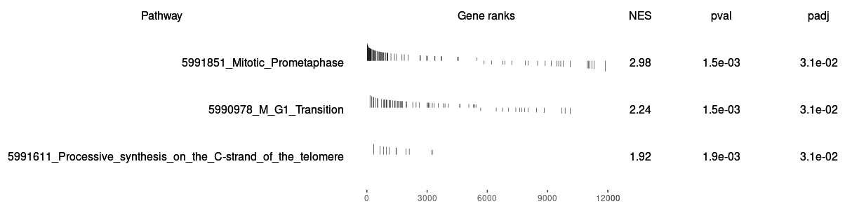
Both two packages have functions for Visualizing their results. Function plotEnrichment is more friendly to customized data. What a surprise is it has plotGseaTable function which from fgsea could show multiple results in a table-like panel. Though this graphic is not fancy but could be very helpful in some situations.

gseaplot(gse, geneSetID = "5991851_Mitotic_Prometaphase")
plotEnrichment(examplePathways[['5991851_Mitotic_Prometaphase']], exampleRanks)

# Example of using gse result
# plotEnrichment(gse@geneSets[['5991851_Mitotic_Prometaphase']], exampleRanks)

plotGseaTable(examplePathways[List], exampleRanks, fgseaRes,  
                  gseaParam=0.5)

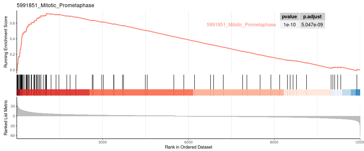
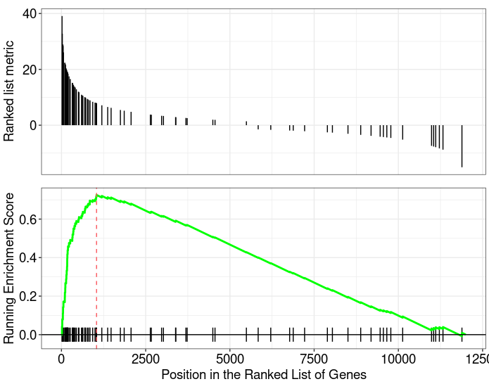
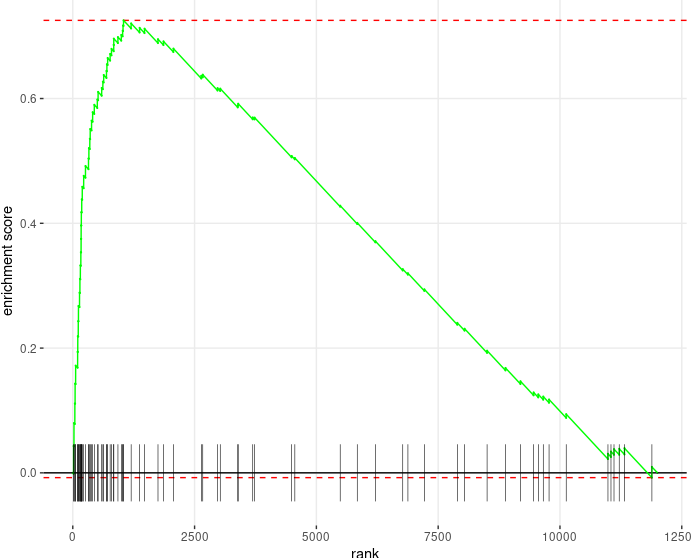
gseaplot from clusterProfiler	plotEnrichment from fgsea

Check the Data Formats and Fabric a group of GeneList & GeneSets

• exampleRanks:

    170942    109711     18124     12775     72148     16010
    -63.33703 -49.74779 -43.63878 -41.51889 -33.26039 -32.77626 

• examplePathways:

    $`186589_Late_stage_branching_morphogenesis_pancreatic_bud_precursor_cells`
    [1] "11925"  "15205"  "21410"  "246086"

The above two lists show a quick view of example data. exampleRanks is an increasing/decreasing numeric vector. examplePathways is a list that contains the name of each set and genes under each set.

An example of generating your own data:

set.seed(1)
GeneList <- sample(seq(-100,100,0.01), 100)
names(GeneList) <- paste("Gene", c(1:100), sep="_")
GeneSet <- append(list(names(GeneList)[1:50]), list(names(GeneList)[40:100]))
names(GeneSet) <- c("Set1", "Set2")

# List table for clusterProfiler
TERM2GENE_exp = ldply(GeneSet, data.frame)
# Sort the GeneList
GeneList <- sort(GeneList, decreasing =  T)
fgseaRes <- fgsea(GeneSet, GeneList, nperm=1000, maxSize=500, minSize = 10)

gse <- GSEA(gene = GeneList ,  TERM2GENE = TERM2GENE_exp, pvalueCutoff = 1)

pathway	pval	padj	ES	NES	nMoreExtreme	size
Set1	0.845140032948929	0.980519480519481	0.20117826706011	0.764831637359588	512	50
Set2	0.980519480519481	0.980519480519481	0.156182133808093	0.582211034023132	603	61

Description	setSize	enrichmentScore	NES	pvalue	p.adjust	qvalues	rank	leading_edge
Set1	50	0.20117826706011	0.750929659683889	0.834633385335413	0.971742543171115	0.971742543171115	34	tags=38%, list=34%, signal=50%
Set2	61	0.156182133808093	0.586558400598972	0.971742543171115	0.971742543171115	0.971742543171115	18	tags=18%, list=18%, signal=38%

Enrichment Plot

library(enrichplot)

gseaplot2(gse, geneSetID = 1, title = gse$Description[1], color = 'salmon', pvalue_table = TRUE)
gseaplot2(gse, geneSetID = 1:7, title = "GSEA", color = 'salmon', pvalue_table = TRUE)

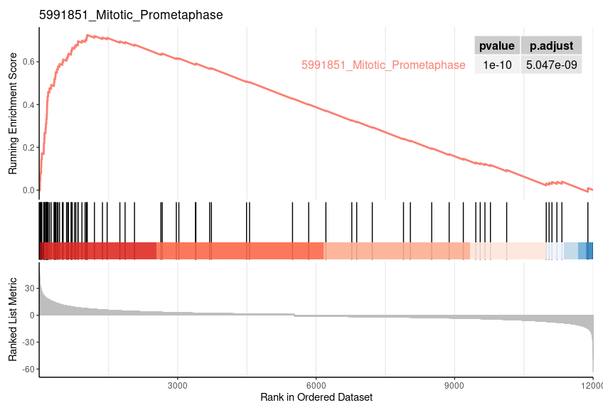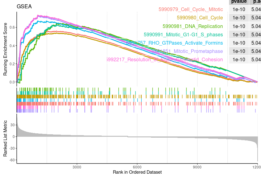
geneSetID = 1	geneSetID = 1:7

What is nPerm

The nominal p value estimates the statistical significance of the enrichment score for a single gene set. However, when you are evaluating multiple gene sets, you must correct for gene set size and multiple hypothesis testing. Because the p value is not adjusted for either, it is of limited value when comparing gene sets.

The FDR is adjusted for gene set size and multiple hypotheses testing while the p value is not. When a top gene set has a small nominal p value and a high FDR value, it generally indicates that it is not as significant when compared with other gene sets in the empirical null distribution. This could be because you do not have enough samples, the biological signal is subtle, or the gene sets do not represent the biology in question very well. On the other hand, the FDR is based on two distributions of all gene sets; if only one of many gene sets is enriched, that gene set is likely to have a high FDR. Finally, a top gene set with a high nominal p value and a low FDR value, generally indicates a negative result: the gene set itself is not significant and other sets are weaker.

In the GSEA report, a p value of zero (0.0) indicates an actual p value of less than 1/number-of-permutations. For example, if the analysis performed 100 permutations, a reported p value of 0.0 indicates an actual p value of less than 0.01. For a more accurate p value, increase the number of permutations performed by the analysis. Typically, you will want to perform 1000 permutations (phenotype or gene_set). (If you attempt to perform significantly more than 1000 permutations, GSEA may run out of memory.)

From: © gsea-msigdb.org

More FAQ could be found at: software.broadinstitute.org

Other things you need to know

• ES (enrichment score): reflects the degree to which a gene-set is overrepresented at the top or bottom of a ranked list of genes.
• NES (normalized enrichment score): NES corrects for differences in ES between gene-sets due to differences in gene-set sizes. It enables to compare the scores of the different tested gene-sets with each other.
  NES = actual ES / mean of all ESs obtained from all random permutations for the single gene-set that is being tested
• nom p-value: The nominal p value estimates the statistical significance of the enrichment score for a single gene set. The p-value is calculated from the null distribution.
  Using gene-set permutation, the null distribution is created by generating, for each permutation, a random gene set the same size as your specified gene set by selecting that number of genes from all of the genes in your expression data set (or pre-ranked list), and then calculating the enrichment score for that randomly selected gene set. The distribution of those enrichment scores across all of the permutations constitutes the null distribution.
• FDR: corrects for multiple hypothesis testing and enable a more correct comparison of the different tested gene-sets with each other.
  • note: for a given gene-set S and observed NES, called NES*, FDR is [% of all NES (including permutations) >= NES*] / [% of all observed NES (=NES for all tested gene-sets) >= NES*]
• relationships between ES, pvalue , NES and FDR:
  • pvalue is calculated from ES
  • FDR is calculated from NES
  • the higher the ES or NES and the lowest the FDR or pvalue
  • NES above 1.4 will usually give significant results

© BADER LAB, 2016