RNN, Recurrent Neural Network

RNN, Recurrent Neural Network

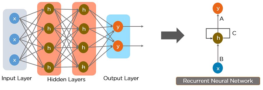
A Recurrent Neural Network (RNN) is a class of artificial neural network that has memory or feedback loops that allow it to better recognize patterns in data. RNNs are an extension of regular artificial neural networks that add connections feeding the hidden layers of the neural network back into themselves - these are called recurrent connections. The recurrent connections provide a recurrent network with visibility of not just the current data sample it has been provided, but also it’s previous hidden state. A recurrent network with a feedback loop can be visualized as multiple copies of a neural network, with the output of one serving as an input to the next. Unlike traditional neural networks, recurrent nets use their understanding of past events to process the input vector rather than starting from scratch every time.

A RNN is particularly useful when a sequence of data is being processed to make a classification decision or regression estimate but it can also be used on non-sequential data. Recurrent neural networks are typically used to solve tasks related to time series data. Applications of recurrent neural networks include natural language processing, speech recognition, machine translation, character-level language modeling, image classification, image captioning, stock prediction, and financial engineering. We can teach RNNs to learn and understand sequences of words. RNNs can also be used to generate sequences mimicking everything from Shakespeare to Linux source code, to baby names.
© NVDIA

Recurrent neural networks have memory to remember important past events, which is essential for successful sequence learning. Regular neural networks have fixed input size, while recurrent networks can handle sequences of any length. They process each element of a sequence one at a time, making them suitable for processing sequential data.

A Sample Example

There is an example from Abid Ali Awan, 2022.
The training data is from kaggle MasterCard Stock Data

# Importing the libraries
import numpy as np
import pandas as pd
import matplotlib.pyplot as plt

from sklearn.preprocessing import MinMaxScaler
from sklearn.metrics import mean_squared_error

from tensorflow.keras.models import Sequential
from tensorflow.keras.layers import Dense, LSTM, Dropout, GRU, Bidirectional
from tensorflow.keras.optimizers import SGD
from tensorflow.random import set_seed

set_seed(455)
np.random.seed(455)

# Read the data
dataset = pd.read_csv(
    "/home/ken/Downloads//Mastercard_stock_history.csv", index_col="Date", parse_dates=["Date"]
).drop(["Dividends", "Stock Splits"], axis=1)
print(dataset.head())

                Open      High       Low     Close     Volume
Date                                                         
2006-05-25  3.748967  4.283869  3.739664  4.279217  395343000
2006-05-26  4.307126  4.348058  4.103398  4.179680  103044000
2006-05-30  4.183400  4.184330  3.986184  4.093164   49898000
2006-05-31  4.125723  4.219679  4.125723  4.180608   30002000
2006-06-01  4.179678  4.474572  4.176887  4.419686   62344000

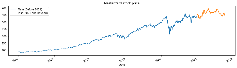
This code is for visualizing the training and testing data. We use the data from the previous year as the training data to predict the data for the last four years.

tstart = 2016
tend = 2020

def train_test_plot(dataset, tstart, tend):
    dataset.loc[f"{tstart}":f"{tend}", "High"].plot(figsize=(16, 4), legend=True)
    dataset.loc[f"{tend+1}":, "High"].plot(figsize=(16, 4), legend=True)
    plt.legend([f"Train (Before {tend+1})", f"Test ({tend+1} and beyond)"])
    plt.title("MasterCard stock price")
    plt.show()

train_test_plot(dataset,tstart,tend)

Detailed explain

The code defines a function `train_test_plot` that takes in a dataset, a start year `tstart`, and an end year `tend`. It plots the `High` column of the dataset for the years between `tstart` and `tend`, and the `High` column of the dataset for the years after `tend+1`.

This function is then called with the `dataset`, `tstart`, and `tend` variables that were previously defined from reading in the Mastercard stock history data.

The resulting plot shows the trend of the Mastercard stock price for the years before `tend+1` (train data) and the years after `tend+1` (test data). The plot helps to visualize how the dataset is split into training and testing sets for model development and evaluation.

def train_test_split(dataset, tstart, tend):
    train = dataset.loc[f"{tstart}":f"{tend}", "High"].values
    test = dataset.loc[f"{tend+1}":, "High"].values
    return train, test
training_set, test_set = train_test_split(dataset, tstart, tend)
sc = MinMaxScaler(feature_range=(0, 1))
training_set = training_set.reshape(-1, 1)
training_set_scaled = sc.fit_transform(training_set)
def split_sequence(sequence, n_steps):
    X, y = list(), list()
    for i in range(len(sequence)):
        end_ix = i + n_steps
        if end_ix > len(sequence) - 1:
            break
        seq_x, seq_y = sequence[i:end_ix], sequence[end_ix]
        X.append(seq_x)
        y.append(seq_y)
    return np.array(X), np.array(y)

n_steps = 60
features = 1
# split into samples
X_train, y_train = split_sequence(training_set_scaled, n_steps)

# Reshaping X_train for model
X_train = X_train.reshape(X_train.shape[0],X_train.shape[1],features)

Detailed explain

The code defines several functions to prepare the dataset for training the RNN model.

The train_test_split function takes in the dataset, tstart, and tend variables and returns the High column values of the dataset for the years between tstart and tend as the training set and the High column values of the dataset for the years after tend+1 as the test set.

The MinMaxScaler function from sklearn.preprocessing is used to scale the training_set values between 0 and 1. Then, the split_sequence function is defined to split the training set into input-output sequences of length n_steps. This function takes in a sequence and the number of time steps to split the sequence into.

Next, n_steps and features are defined as 60 and 1, respectively. The split_sequence function is then called to split the training_set_scaled into X_train (input sequences) and y_train (output sequences) for the RNN model.

Finally, X_train is reshaped to a 3D tensor to match the input shape required by the RNN model, with dimensions (number of samples, number of time steps, number of features). The number of samples is inferred from the input data, number of time steps is set to n_steps, and number of features is set to 1.

In this code, we only focus on the “High” column. After splitting the data into training_set and test_set using a predefined function, they are still one-dimensional with lengths of 1259 and 195, respectively. Next, we need to reshape the training set and scale it using MinMaxScaler.

We then define a number of steps (n_steps) for the input sequence. This is similar to defining a sliding window, with the window size determined by the number of steps. Based on the features of this window, we can predict the information beyond the window.

LSTM Model

# The LSTM architecture
model_lstm = Sequential()
model_lstm.add(LSTM(units=125, activation="tanh", input_shape=(n_steps, features)))
model_lstm.add(Dense(units=1))
# Compiling the model
model_lstm.compile(optimizer="RMSprop", loss="mse")

model_lstm.summary()
model_lstm.fit(X_train, y_train, epochs=50, batch_size=32)

dataset_total = dataset.loc[:,"High"]
inputs = dataset_total[len(dataset_total) - len(test_set) - n_steps :].values
inputs = inputs.reshape(-1, 1)
#scaling
inputs = sc.transform(inputs)

# Split into samples
X_test, y_test = split_sequence(inputs, n_steps)
# reshape
X_test = X_test.reshape(X_test.shape[0], X_test.shape[1], features)
#prediction
predicted_stock_price = model_lstm.predict(X_test)
#inverse transform the values
predicted_stock_price = sc.inverse_transform(predicted_stock_price)

def plot_predictions(test, predicted):
    plt.plot(test, color="gray", label="Real")
    plt.plot(predicted, color="red", label="Predicted")
    plt.title("MasterCard Stock Price Prediction")
    plt.xlabel("Time")
    plt.ylabel("MasterCard Stock Price")
    plt.legend()
    plt.show()


def return_rmse(test, predicted):
    rmse = np.sqrt(mean_squared_error(test, predicted))
    print("The root mean squared error is {:.2f}.".format(rmse))

plot_predictions(test_set,predicted_stock_price)

return_rmse(test_set,predicted_stock_price)

Detailed explain

The code is building a LSTM (Long Short-Term Memory) neural network model for time-series forecasting.

First, the code splits the dataset into training and testing sets using a specified time period. It then applies feature scaling to the training set using MinMaxScaler, which scales the data to a range between 0 and 1.

The function split_sequence is defined to prepare the training data into input-output pairs. Given a sequence of data points, this function divides the data into input sequences (X) of length n_steps and the corresponding output values (y).

The LSTM model is defined using the Sequential class from Keras. It has one LSTM layer with 125 units and a tanh activation function. The output from the LSTM layer is then passed to a Dense layer with one unit. The model is compiled with the RMSprop optimizer and mean squared error (mse) loss function.

After defining the model, the training set is used to fit the model for 50 epochs with a batch size of 32.

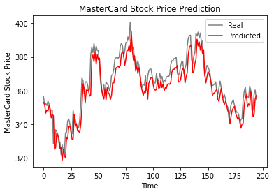
Next, the testing set is prepared by selecting the required number of time steps from the end of the dataset, scaling it, and then splitting it into input-output pairs using the same split_sequence function. The input sequence is then reshaped into a 3D format that can be input into the LSTM model. Finally, the model is used to make predictions on the testing set, and the predictions are inverse transformed to get the actual stock prices.

GRU Model

model_gru = Sequential()
model_gru.add(GRU(units=125, activation="tanh", input_shape=(n_steps, features)))
model_gru.add(Dense(units=1))
# Compiling the RNN
model_gru.compile(optimizer="RMSprop", loss="mse")

model_gru.summary()
model_gru.fit(X_train, y_train, epochs=50, batch_size=32)
GRU_predicted_stock_price = model_gru.predict(X_test)
GRU_predicted_stock_price = sc.inverse_transform(GRU_predicted_stock_price)
plot_predictions(test_set, GRU_predicted_stock_price)
return_rmse(test_set,GRU_predicted_stock_price)

Detailed explain

The code is defining and training a GRU (Gated Recurrent Unit) model for predicting stock prices.

First, the model is defined using the Keras Sequential API. The model has one GRU layer with 125 units and “tanh” activation function, and a Dense output layer with one unit. The model is then compiled using “RMSprop” optimizer and “mse” loss function.

The model is trained using the training data, X_train and y_train, with 50 epochs and a batch size of 32.

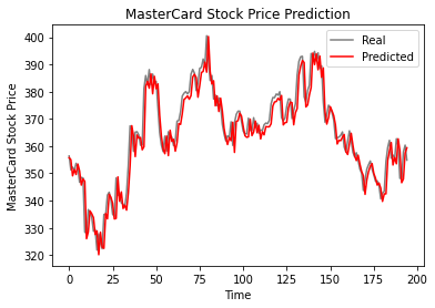
Then, the model is used to predict the stock prices for the test set using the predict method. The predicted prices are then inverse-transformed using the MinMaxScaler to obtain the actual stock prices.

Finally, the predicted prices are plotted against the actual prices using the plot_predictions function and the root-mean-square error (RMSE) is computed using the return_rmse function.

RNN in Action

Prepair the functions

def split_sequence(sequence, n_steps):
    X, y = list(), list()
    for i in range(len(sequence)):
        end_ix = i + n_steps
        if end_ix > len(sequence) - 1:
            break
        seq_x, seq_y = sequence[i:end_ix], sequence[end_ix]
        X.append(seq_x)
        y.append(seq_y)
    return np.array(X), np.array(y)
def Data_prepare(training_set, n_steps = 60, features =1):
    #sc = MinMaxScaler(feature_range=(0, 1))
    training_set = training_set.reshape(-1, 1)
    #training_set_scaled = sc.fit_transform(training_set)
    # split into samples
    X_train, y_train = split_sequence(training_set_scaled, n_steps)

    # Reshaping X_train for model
    X_train = X_train.reshape(X_train.shape[0],X_train.shape[1],features)
    return X_train, y_train

import pandas as pd
Data = "/media/ken/DATA/tracking_test/WT_court10min_ID.csv"
TB = pd.read_csv(Data, index_col=0)

# select the Fly_8 as an example
#for ID in TB.ID.unique()[:12]:
ID = "Fly_8"
training_set_X = TB.X[TB.ID==ID][:2000].to_numpy()
test_set_X = TB.X[TB.ID==ID][2000:3000].to_numpy()
training_set_Y = TB.Y[TB.ID==ID][:2000].to_numpy()
test_set_Y = TB.Y[TB.ID==ID][2000:3000].to_numpy()

plt.plot(training_set_X, training_set_Y)
plt.plot(test_set_X, test_set_Y)
plt.show()

n_steps = 60
features = 2

training_set = TB[["X", "Y"]][TB.ID==ID][:2000].to_numpy()
X_train, y_train = split_sequence(training_set, n_steps)
X_train = X_train.reshape(X_train.shape[0],X_train.shape[1],features)

test_set = TB[["X", "Y"]][TB.ID==ID][2000:3000].to_numpy()
X_test, y_test = split_sequence(test_set, n_steps)
X_test = X_test.reshape(X_test.shape[0],X_test.shape[1],features)


model_gru = Sequential()
model_gru.add(GRU(units=125, activation="tanh", input_shape=(n_steps, features)))
model_gru.add(Dense(units=2))
# Compiling the RNN
model_gru.compile(optimizer="RMSprop", loss="mse")

model_gru.summary()
model_gru.fit(X_train, y_train, epochs=50, batch_size=32)

GRU_predicted_stock_price = model_gru.predict(X_test)
#GRU_predicted_stock_price = sc.inverse_transform(GRU_predicted_stock_price)

plt.plot(GRU_predicted_stock_price[:,0], GRU_predicted_stock_price[:,1])
plt.plot(test_set[:,0], test_set[:,1])
plt.show()


Predict = []
Track = X_train[-1] 
for i in range(1000):
    Predict += model_gru.predict(np.array([Track])).tolist()
    Track = np.concatenate([Track[1:], [Predict[-1]]])

plt.plot(np.array(Predict)[:,0], np.array(Predict)[:,1])
plt.plot(GRU_predicted_stock_price[:,0], GRU_predicted_stock_price[:,1])
plt.plot(test_set[:,0], test_set[:,1])
plt.show()


# plot for other fly



test_set = TB[["X", "Y"]][TB.ID==ID].to_numpy()
X_test, y_test = split_sequence(test_set, n_steps)
X_test = X_test.reshape(X_test.shape[0],X_test.shape[1],features)
plt.plot(GRU_predicted_stock_price[:,0], GRU_predicted_stock_price[:,1])
plt.plot(test_set[:,0], test_set[:,1])
plt.show()