Response Surface Methodology in R

Response Surface Methodology in R (rsm)

Introduction of RSM and rsm pacakge

Response-surface methodology comprises a body of methods for exploring for optimum operating conditions through experimental methods.

The rsm package for R (R Development Core Team 2009^[1]) provides several functions to facilitate classical response-surface methods.

Commercial Software for rsm:

• Design-Expert
• JMP
• Statgraphics

rsm covers only the most standard first-and second order designs and methods for one response variable.

desirability package (Kuhn 2009) may be used in conjunction with predictions obtained using the rsm package

Install

install.packages('rsm')

Started With

library("rsm")
ChemReact

Table ChemReact:

Time   Temp Block Yield
1  80.00 170.00    B1  80.5
2  80.00 180.00    B1  81.5
3  90.00 170.00    B1  82.0
4  90.00 180.00    B1  83.5
5  85.00 175.00    B1  83.9
6  85.00 175.00    B1  84.3
7  85.00 175.00    B1  84.0
8  85.00 175.00    B2  79.7
9  85.00 175.00    B2  79.8
10 85.00 175.00    B2  79.5
11 92.07 175.00    B2  78.4
12 77.93 175.00    B2  75.6
13 85.00 182.07    B2  78.5
14 85.00 167.93    B2  77.0

coded.date

The first block, ChemReact1, uses factor settings of Time = 85 ± 5 and Temp = 175 ± 5, with three center points. Thus, the coded variables are x1 = (Time − 85)=5 and x1 = (Temp − 175)=5.

CR1 <- coded.data(ChemReact1, x1 ~ (Time - 85)/5, x2 ~ (Temp - 175)/5)
CR1

Time Temp Yield
1   80  170  80.5
2   80  180  81.5
3   90  170  82.0
4   90  180  83.5
5   85  175  83.9
6   85  175  84.3
7   85  175  84.0

Data are stored in coded form using these coding formulas ...
x1 ~ (Time - 85)/5
x2 ~ (Temp - 175)/5

## data frame was used to plot
as.data.frame(CR1)

des1 <- ccd (y1 + y2 ~ A + B + C + D,
  generators = E ~ - A * B * C * D, n0 = c(6, 1))

des10 <- ccd( ~ A + B + C + D + E,
  blocks = Blk ~ c(A * B * C, C * D * E), n0 = c(2, 4))

par(mfrow=c(1,2))
varfcn(des10, ~ Blk + SO(A,B,C,D,E), dist = seq(0, 3, by=.1))
varfcn(des10, ~ Blk + SO(A,B,C,D,E), dist = seq(0, 3, by=.1), contour = TRUE)

ccd(2, n0 = c(1,1), inscribed=TRUE, randomize=FALSE)

run.order std.order   x1.as.is   x2.as.is Block
1          1         1 -0.7071068 -0.7071068     1
2          2         2  0.7071068 -0.7071068     1
3          3         3 -0.7071068  0.7071068     1
4          4         4  0.7071068  0.7071068     1
5          5         5  0.0000000  0.0000000     1
6          1         1 -1.0000000  0.0000000     2
7          2         2  1.0000000  0.0000000     2
8          3         3  0.0000000 -1.0000000     2
9          4         4  0.0000000  1.0000000     2
10         5         5  0.0000000  0.0000000     2

Data are stored in coded form using these coding formulas ...
x1 ~ x1.as.is
x2 ~ x2.as.is

CR1.rsm <- rsm(Yield ~ FO(x1, x2), data = CR1)
summary(CR1.rsm)

CCD (Central-Composite Design)

One of the most popular response-surface designs is the central-composite design (CCD), due to Box and Wilson (1951)^[2].

it works as the codes show below, but I didn’t figure out how exactly why = =

Fitting a Response-Surface Model

library(rsm)

CR1 <- coded.data(ChemReact1, x1 ~ (Time - 85)/5, x2 ~ (Temp - 175)/5)

CR1.rsm <- rsm(Yield ~ FO(x1, x2), data = CR1)
CR1.rsmi <- update(CR1.rsm, . ~ . + TWI(x1, x2))
CR2 <- djoin(CR1, ChemReact2)
CR2.rsm <- rsm(Yield ~ Block + SO(x1, x2), data = CR2)

png('image.png',w=450, h= 1000)
par(mfrow=c(3,1))
image(CR1.rsm, x1~ x2)
image(CR1.rsmi, x1~ x2)
image(CR2.rsm, x1~ x2)
dev.off()

png('persp.png',w=450, h= 1000)
par(mfrow=c(3,1))
persp(CR1.rsm, x1~ x2, col='blue', contours = list(z='top',col='orange'))
persp(CR1.rsmi, x1~ x2, col='blue', contours = list(z='top',col='orange'))
persp(CR2.rsm, x1~ x2, col='blue', contours = list(z='top',col='orange'))  
dev.off()

Images:

image(CR1.rsm, x1~ x2) image(CR1.rsmi, x1~ x2) image(CR2.rsm, x1~ x2)	persp(CR1.rsm, x1~ x2, col=‘blue’, contours = list(z=‘top’,col=‘orange’)) persp(CR1.rsmi, x1~ x2, col=‘blue’, contours = list(z=‘top’,col=‘orange’)) persp(CR2.rsm, x1~ x2, col=‘blue’, contours = list(z=‘top’,col=‘orange’))

More about this codes:
Video tutorial: Chris Mack 2016
Codes: Chris Mack 2016

Click to see the explanation of codes

#--------------------------------------#
#--- Response Surface Modeling in R ---#
#--------------------------------------#

#First, install and load the "rsm" package

# install.packages("rsm")
library(rsm)

# Example generating a Box-Behnken design with three factors and two center points (no)
bbd(3, n0 = 2, coding = list(x1 ~ (Force - 20)/3, x2 ~ (Rate - 50)/10, x3 ~ Polish - 4))


# Example data set
data = ChemReact
plot(data)


# The data set was collected in two blocks.
# Block1 is a 2-level, two-factor factorial design with three repeated center points.
# Block 2 is the Central Composite Design (circomscribed) with 3 center points.
# The variables are Time = 85 +/- 5 and Temp = 175 +/- 5,
# Thus, the coded variables are  x1 = (Time-85)/5 and x2 = (Temp-175)/5
CR <- coded.data(ChemReact, x1 ~ (Time - 85)/5, x2 ~ (Temp - 175)/5)
CR[1:7,]

# Note: If the data are already coded, use as.coded.data() to convert to the proper coded data object

# Let's work as though the first block (full factorial) has been finished,
# and we'll fit a linear model, first order (FO), to it (Yield is the response)
CR.rsm1 <- rsm(Yield ~ FO(x1, x2), data = CR, subset = (Block == "B1"))
summary(CR.rsm1)

#The fit is not very good.  Let's include the interaction term (TWI) and update the model, or start over with a new model (these two lines do the same thing)
CR.rsm1.5 <- update(CR.rsm1, . ~ . + TWI(x1, x2))
CR.rsm1.5 <- rsm(Yield ~ FO(x1, x2)+TWI(x1, x2), data = CR, subset = (Block == "B1"))
summary(CR.rsm1.5)
#This is no better!  The reason is the strong quadratic response, with the peak near the center.

# Now let's assume the second block has been collected.  We use the SO (second order) function, which includes FO and TWI
CR.rsm2 <- rsm(Yield ~ Block + SO(x1, x2), data = CR)
summary(CR.rsm2)

# The secondary point is a maximum (both eigenvalues are negative) and within the experimental design range (no extrapolation)

# Also note that the block is significant, meaning that the processes shifted between the first set of data and the second.  This is not good.  The coefficient is -4.5, meaning the yield shifted down by 4.5% between the two blocks - a more significant effect than either temperatue or time!  This is most easily seen by looking at the repeat center points.

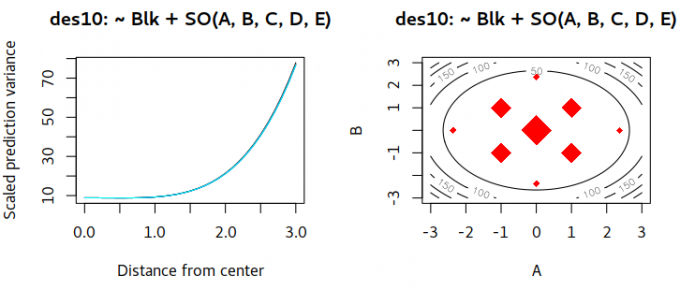
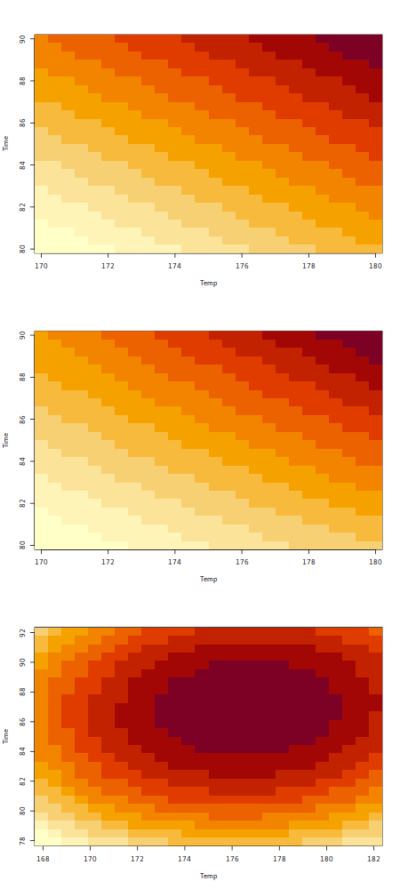
# We can plot the fitted response as a contour plot.
contour(CR.rsm2, ~ x1 + x2, at = summary(CR.rsm2)$canonical$xs)

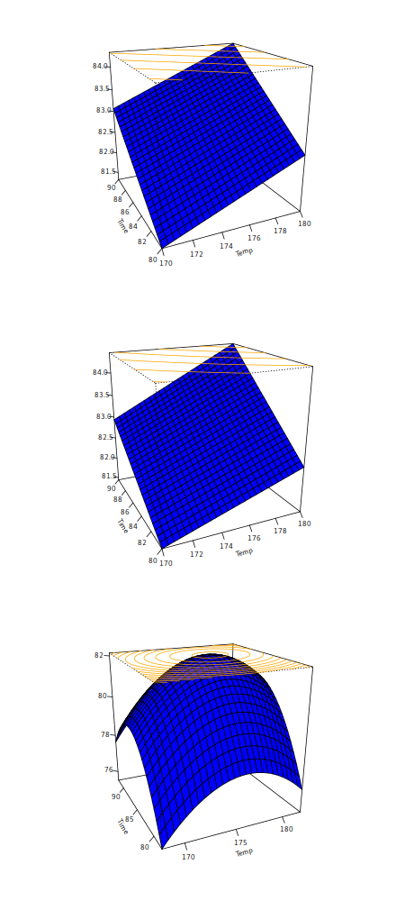
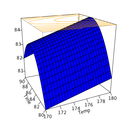
On the other hand:

An other algorithm to plot the surface by lm which explained by Resseel V. Lenth 2010^[3]

A.lm <- lm( Yield ~ poly(Time, Temp, degree =2),data=ChemReact1)
image(A.lm, Time~ Temp)
contour(A.lm, Time~ Temp)
persp(A.lm, Time~ Temp, col='blue', contours = list(z='top',col='orange'))  

It’s clearly different from the result above.

st=>start: Table sp1=>operation: coded.date:>#step1 e=>end: End:>http://www.google.com op1=>operation: My Operation|past op2=>operation: Stuff|current sub1=>subroutine: 这啥啊|invalid cond=>condition: Yes or No?|approved:>http://www.google.com c2=>condition: Good idea|rejected io=>inputoutput: catch something...|request st->sp1(right) cond(yes, right)->c2 cond(no)->sub1(left)->op1 c2(yes)->io->e c2(no)->op2(right)->op1{"theme":"simple","scale":1,"line-width":2,"line-length":50,"text-margin":10,"font-size":12}

---

1. R Development Core Team (2009). R: A Language and Environment for Statistical Computing. R Foundation for Statistical Computing, Vienna, Austria. ISBN 3-900051-07-0, URL http://www.R-project.org/. ↩︎

2. Box GEP, Wilson KB (1951). “On the Experimental Attainment of Optimum Conditions.” Journal of the Royal Statistical Society B, 13, 1-45. ↩︎

3. Surface Plots in the rsm Package ↩︎