Statistic for Data Scientists 1| | Reading Notes

Estimates of Location

Mean; Weighter mean, Median, Weighted median, Trimmed mean, Robust, Outlier.

Mean	$\overline{x} = \frac{\sum_ i^ n x_ i}{n}$
Trimmed mean	$ \overline{x} = \frac{\sum_ {i=p+1} ^{n-p} x_ {(i)}}{n-2p}$
Weighted mean	$\overline{x}_ w = \frac{\sum_ {i=1} ^ n w_ i x_ i}{\sum_ i ^ n w_ i }$

Estimates of Variability

Term	Synonyms	Description
Deviations	errors, residuals	The difference between the observed values and the estimate of location
Varuance	mean-squared-error	THe sum of squared deviations from the mean divided by $n - 1$ where n is the number of data values
Standard deviation	l2-norm, Eucliden norm	The square root of the variance.
Mean absolute deviation	l1-norm, Manhattan norm	The mean of the absolute value of the deviations from the mean.
Median absolute deviation from the median		The median of the absolute value of the deviations from the median
Range		The difference between the largest and the smallest value in a data set.
Order statistics	Ranks	Metrics based on the date values sorted from smallest to biggest.
Precentile	quantile	The value such that P percent of the values take on this value or less ad (100-P) percent take on this value or more.
Interquartile range	IQR	The differentce between the 75th percentile and the 25th percentile.

Deviation

Mean absolution deviation	$\frac{\sum ^ n _ {i=1} | x_ i - \overline{x}|}{n}$
Variance	$s^ 2 = \frac{\sum (x - \overline{x})^ 2}{n-1}$
Standard deviation	$s = \sqrt{s^ 2}$

For Mean absolution deviation:

List <- c(1,2,3,4,5)
MAD <- function(List){
  Tmp = 0
  for( num in List){
    Tmp = Tmp + abs(num - mean(List))
  }
  Result = Tmp/length(List)
  return(Result)
}

'''
in R mad()

Instated of Tmp/length(List), in function mad(),
it using Tmp/(length(List)-1)
'''

For Variance:

List <- c(1,2,3,4,5)
VAR <- function(List){
  Tmp = 0
  for( num in List){
    Tmp = Tmp + (num - mean(List))^2
  }
  Result = Tmp/(length(List)-1)
  return(Result)
}
# var() in R

For Standard Deviation

List <- c(1,2,3,4,5)
SD <- function(List){
  Tmp = 0
  for( num in List){
    Tmp = Tmp + (num - mean(List))^2
  }
  Result = Tmp/(length(List)-1)
  Result = sqrt(Result)
  return(Result)
}

# sd() in R

Why n - 1

In the intuitive denominator of n in the variance formulation, it would underestimate the true variance and the standard deviation. This is referred to as a biased estimate.
If you divided by $n-1$, the standard deviation becomes an unbiased estimate.

Test: function SD() and sd()
SD() is using $n$, which is biased estimate,
sd() is the base function of R, which use unbiased estimate.

SD <- function(List){
  Tmp = 0
  for( num in List){
    Tmp = Tmp + (num - mean(List))^2
  }
  Result = Tmp/length(List)
  Result = sqrt(Result)
  return(Result)
}

Test <- function(List, i){
  A = SD(List)
  B = sd(List)
  C = mad(List)
  D = var(List)
  Result = "|"
  List_str = "$c(1,2,3,4,5,6,7,8,9,10)"
  List_str_tmp = paste(List_str, "^ {",(1+ i/10),"}$",sep="")
  Result = paste(Result, List_str_tmp, sep = "")
  Result = paste(Result, "|",A,"|",B,"|", C,"|", D, "|",sep = "")
  print(C)
  #print(Result)
  return(data.frame(A, B,C,D))
}
TB = data.frame()
for(i in c(0:10)){
  List <- c(1,2,3,4,5,6,7,8,9,10)
  List <- List ^(1+ i/10)
  TB = rbind(TB, Test(List, i))
}

List	SD	sd	mad	var
$c(1,2,3,4,5,6,7,8,9,10)^ {1}$	2.87228132326901	3.02765035409749	3.7065	9.16666666666667
$c(1,2,3,4,5,6,7,8,9,10)^ {1.1}$	3.71464847156818	3.91558329233956	4.81903250216669	15.3317925192487
$c(1,2,3,4,5,6,7,8,9,10)^ {1.2}$	4.77822834483576	5.03669491668582	6.21842448942231	25.3682956837688
$c(1,2,3,4,5,6,7,8,9,10)^ {1.3}$	6.1203589266995	6.45142476870465	7.97443123015422	41.6208815462559
$c(1,2,3,4,5,6,7,8,9,10)^ {1.4}$	7.81312940963156	8.23576152936081	10.1733320771185	67.8277679684995
$c(1,2,3,4,5,6,7,8,9,10)^ {1.5}$	9.94716631430172	10.4852339392319	12.9217964296424	109.940130760421
$c(1,2,3,4,5,6,7,8,9,10)^ {1.6}$	12.6363910464884	13.3199257038206	16.2215684620237	177.420420755302
$c(1,2,3,4,5,6,7,8,9,10)^ {1.7}$	16.0239981545644	16.8907771302528	19.8184284109695	285.298352063871
$c(1,2,3,4,5,6,7,8,9,10)^ {1.8}$	20.289967545938	21.3875036986871	24.1444312624589	457.425314461353
$c(1,2,3,4,5,6,7,8,9,10)^ {1.9}$	25.6605043589986	27.0485465610381	29.3423269903854	731.623871064649
$c(1,2,3,4,5,6,7,8,9,10)^ {2}$	32.4199012953463	34.1735765370459	35.5824	1167.83333333333

(Click the tag “var” below to dismiss the line “var”)

Percentile

Percentile was widely used in boxplot (interquartile range or IQR). It was more sensitive to the outliers, and the massive calculation also restricted its applicability since it needs sorting the data set though there are a machine learning algorithms to get an approximate percentile very quickly^[1].

When the data (n is even):
$$
100 \frac{j}{n} \le P < 100\frac{j+1}{n}
$$

Formally, the percentile is the weighted average:

$$
P = (1 - w) x _ {(j)} + wx_ {j + 1}
$$

IQR in R:

$$
IQR(x) = quantile(x, 3/4) - quantile(x, 1/4)
$$

R

IQR(c(1,2,3,4,5,6,7,8,9,10))

[1] 4.5

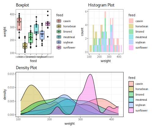
Variation illustration

R

library(ggplot2)
library(patchwork)

P1 <- ggplot(chickwts, aes(feed, weight, fill = feed, group = feed)) +
    geom_point()  + geom_boxplot( alpha = 0.4) + theme_bw()+
    labs( title= "Boxplot")
P2 <- ggplot(chickwts, aes(weight, fill = feed, group = feed)) +
    geom_density(alpha = 0.4) + theme_bw() +
    labs( title= "Density Plot")
P3 <- ggplot(chickwts, aes(weight, fill = feed, group = feed)) +
    geom_histogram( alpha = 0.4)+ theme_bw()+
    labs( title= "Histogram Plot")

(P1|P3) /P2  

@ Karobben

---

1. Qi Zhang and Wei Wang. 2007. A Fast Algorithm for Approximate Quantiles in High Speed Data Streams. In Proceedings of the 19th International Conference on Scientific and Statistical Database Management (SSDBM '07). IEEE Computer Society, USA, 29. DOI:https://doi.org/10.1109/SSDBM.2007.27 ↩︎