BioStatistics with R/Python: Block 1

Biomedical Statistics and Data Analysis

Normal Distribution

(PS: If you don’t have any other information, or have too few data points to test the assumption, it is acceptable to assume a Gaussian distribution.)

$$
Pr(X = x|\mu, σ^ 2) = p ( x | \mu , σ^ 2) = \frac{A}{\sigma \sqrt{ 2 \pi}} e^{- \frac{1}{2}(\frac{x-\mu}{\sigma})^ 2}
$$

A = Area under curve
μ = mean
σ = standard deviation

Normal distribution codes for python

© R CODER

In R, there are few functions for calculate normal distribution related values.
Let’s say, the μ = 0, σ = 1, (as the plot above)
than, we have:
the probability of x is dnorm,
the Z is pnorm. The size of blue area
qnorm: inverse cdf function (Confidence Intervals, CI), the reversed value of the pnorm

dnorm(0,   mean=0, sd=1)
pnorm(0,   mean=0, sd=1)
qnorm(0.5, mean=0, sd=1)

[1] 0.5
[1] 0.3989423
[1] 0

CI calculate ®

CI <- function(A, alpha){
  alpha = 1- alpha
  sample.mean <- mean(A)
  sample.n <- length(A)
  sample.sd <- sd(A)
  sample.se <- sample.sd/sqrt(sample.n)
  print(sample.se)
  degrees.freedom = sample.n - 1
  t.score = qt(p=alpha/2, df=degrees.freedom,lower.tail=F)
  print(t.score)
  margin.error <- t.score * sample.se
  lower.bound <- sample.mean - margin.error
  upper.bound <- sample.mean + margin.error
  print(c(lower.bound,upper.bound))
}

A <- c(12, 3, 4, 2, 42, 4, 42, 524, 5)

CI(A, 0.90)
CI(A, 0.95)
CI(A, 0.99)

rnorm() function for data simulation

from scipy import stats
import numpy as np

rng = np.random.default_rng()
pts = 1000
a = rng.normal(0, 1, size=pts)
b = rng.normal(2, 1, size=pts)
x = np.concatenate((a, b))
k2, p = stats.normaltest(x)
alpha = 1e-3
print("p = {:g}".format(p))
p = 8.4713e-19
if p < alpha:  # null hypothesis: x comes from a normal distribution
    print("The null hypothesis can be rejected")
else:
    print("The null hypothesis cannot be rejected")
The null hypothesis can be rejected

codes for python, 2

Shapiro-Wilk Test

# Shapiro-Wilk Test
from numpy.random import seed
from numpy.random import randn
from scipy.stats import shapiro
# seed the random number generator
seed(1)
# generate univariate observations
data = 5 * randn(100) + 50
# normality test
stat, p = shapiro(data)
print('Statistics=%.3f, p=%.3f' % (stat, p))
# interpret
alpha = 0.05
if p > alpha:
  print('Sample looks Gaussian (fail to reject H0)')
else:
  print('Sample does not look Gaussian (reject H0)')

Shapiro in R

shapiro.test(my_data$len)

    Shapiro-Wilk normality test
data:  my_data$len
W = 0.96743, p-value = 0.1091

note

From the output, the p-value > 0.05 implying that the distribution of the data are not significantly different from normal distribution. In other words, we can assume the normality.

D’Agostino’s K² Test (most widely and used by GraphPad)

# D'Agostino and Pearson's Test
from numpy.random import seed
from numpy.random import randn
from scipy.stats import normaltest
# seed the random number generator
seed(1)
# generate univariate observations
data = 5 * randn(100) + 50
# normality test
stat, p = normaltest(data)
# Stat is k^2
print('Statistics=%.3f, p=%.3f' % (stat, p))
# interpret
alpha = 0.05
if p > alpha:
  print('Sample looks Gaussian (fail to reject H0)')
else:
  print('Sample does not look Gaussian (reject H0)')

Anderson-Darling Test

# Anderson-Darling Test
from numpy.random import seed
from numpy.random import randn
from scipy.stats import anderson
# seed the random number generator
seed(1)
# generate univariate observations
data = 5 * randn(100) + 50
# normality test
result = anderson(data)
print('Statistic: %.3f' % result.statistic)
p = 0
for i in range(len(result.critical_values)):
  sl, cv = result.significance_level[i], result.critical_values[i]
  if result.statistic < result.critical_values[i]:
    print('%.3f: %.3f, data looks normal (fail to reject H0)' % (sl, cv))
  else:
    print('%.3f: %.3f, data does not look normal (reject H0)' % (sl, cv))

PS: 10 Normality Tests in Python (Step-By-Step Guide 2020)

SD and SEM

$$
σ = \sqrt{
\frac {\sum_ N (X_ i - μ)^ 2} { N -1 }
}
$$

$$
sem = \frac{σ}{\sqrt{N}}
$$

SD

• Describes the width of the parent population as estimated from the scatter in the sample measurements. (For example, when the width of the parent population reflects actual variation of the measured quantity more than in reflects experimental uncertainty)
• Does not decrease with more measurements
• Should be used when the width of the parent distribution is important to
  your audience.

SEM

• Describes the uncertainty in the measured value of the mean
• Decreases with more measurements
• Should be used when the accuracy in the measured mean is more important to your audience that the width of the parent population. (For example, when most of the width of the parent population is due to experimental uncertainties)

Always give the sample size so your reader can convert

Rules for expressing means and uncertainties

• Express your data with the last significant digit equal to the precision of your measurement.
• Plot a histogram to see the distribution. Also test whether your data are distributed in a Gaussian manner.
• Present uncertainties as standard deviations if the width of the parent population is important or standard errors if the precision of the measured mean is important. Always define error (SD, SEM) and provide sample number so readers can convert.
• Keep in mind that experiments with small sample sizes are much more variable and have higher uncertainties.

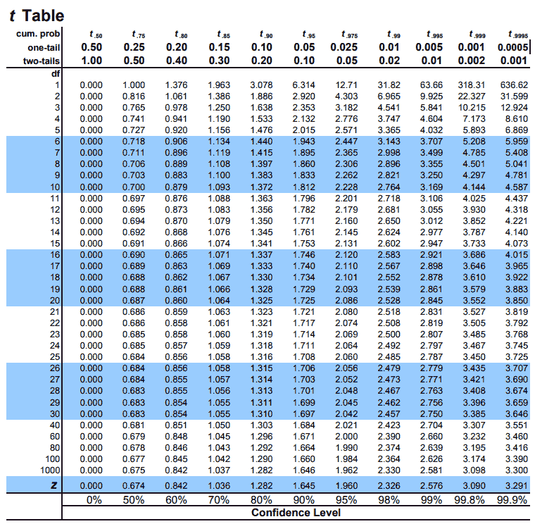
Lecture 3 The t-table

The t distribution is a probability distribution that we can use to express confidence intervals of a mean.

$$
t_ i = \frac{\overline{X_ i} - \mu_ {parent}}{σ/\sqrt{N}}
$$

Interpretation: The deviation of sample mean and parent mean divided by SEM

T Distributuin

For analyze statistical data from small sample.

When measure the small sample Normal distribution, you didn’t get the Gaussine distribution, you get t distribution.

© tdistributiontable.com

dt(x, df, ncp, log = FALSE)
pt(q, df, ncp, lower.tail = TRUE, log.p = FALSE)
qt(p, df, ncp, lower.tail = TRUE, log.p = FALSE)
rt(n, df, ncp)

# two tailed T to P:
T = 2.085963
N = 20
pt(T, df=N-1, lower.tail=FALSE)*2
# Two tailed P to T:
X= 0.05
N = 20
qt(X/2, df=N-1, lower.tail=FALSE)

How to use the T table

In the t table, the index is the degrees of freedom, which is N - 1 (N is the sample size).

For retrieve the rows of the T table:

• Rows = N -1!!! That’s means, when your sample size is 4, you should looking into row 3!

T table related examples:
dummies.com

Confidence Interval (CI) = ±t × SEM

The Confidence Interval (CI) is the range of possible means over which there is a specified probability of observing a similarly measured value.
CI is another way of expressing the uncertainty in a mean.

To calculate a confidence interval (CI):

1. Choose what confidence level you want (95% is typical)
2. p is the probability. Equals 1-confidence level. 95% mean p=0.05
3. Determine the t-value (t*) from a t-table using dF and p
4. Calculate CI using the equation above
5. When you express a CI, make sure the readers knows probability and N

Example:

You measured 8.72 ± 1.21 (SD, N=7) . What is the 99% CI?

1. Calculate $SE = SD/\sqrt7$ = 0.46
2. Determine t (for p=0.01 and dF=6) t= 3.71 (t-table)
   • in r:

   X= 0.01; N = 7
   qt(X/2, df = N-1, lower.tail = F)
   [1] 3.707428

3. Calculate CI = t*SE = 3.17*0.48 = 1.78

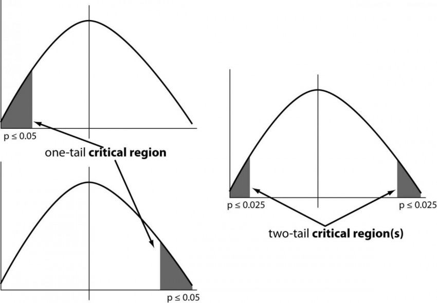
One sided (one tailed) versus two-sided confidence intervals

© Sunil Ray; 2015

Two tailed probabilities are almost always better than one-tailed probabilities because they are more conservative (less likely to lead you to mistakenly claim a positive correlation) and because they do not require any assumption about the sign of the deviation between the actual and measured value.

For symmetrical distributions (Gaussian, t-distribution, etc) the two-tailed probability is twice the one-tailed probability.

Divide probability in a t-table by 2 to convert two-tailed to one-tailed.
Multiple probability by 2 to covert one-tailed to two-tailed.

The p-value

The null hypothesis (H_o) is a hypothetical value of the mean of the parent population. Typically it is the value you would expect to observe if the parameter or conditions of interest have no effect on your measured parameter.

Statistical tests are used to support or disprove the null hypothesis.

The p-value is the probability that you have obtained a difference between your results and the null hypothesis as large as you did observe strictly by chance. In other words, it is the probability of obtaining obtained your results if the null hypothesis was true.

Confidence Intervals and p-values are connected

α is the cutoff that we chose for statistical significance. The ends of the 1-α CI define the values of the null hypothesis that fall exactly at p=α.

A CI defines the range of hypothetical values that have probabilities larger than α, and thus are not significant. Values outside the confidence interval have p-values smaller than α and thus are significant.

$t = \frac{|(H_0 - μ)|}{SE}$
$t = |(H_ 0 -μ)|\sqrt{N}/ sd$
$sd = |(H_ 0 -μ)|\sqrt{N}/t $
$sd = |(0 - )|$

Examples:

Mesurement: 1.235, 2.1254, 3.8926, 1.0022, 0.9880, 2.9876, 1.4350
Your null hypothesis is that the enzyme expression is 1.0.
Do your data disprove the Null hypothesis (H₀)?

A <- c(1.235, 2.1254, 3.8926, 1.0022, 0.9880, 2.9876, 1.4350)
# Step 1: Test the Gaussian?
shapiro.test(A) # p = 0.1528
# Step 2: Calculate mean, SD, SE
mean(A); sd(A); sd(A)/sqrt(length(A))
1.952257 1.116636 0.4220488
# Step 3: Calculate a t-value for the difference between the measured mean and the null hypothesis.
# t = |(H~0~ - μ)/SE| = (1 – 1.9923)/0.422 = 2.35
# Step 4: Look up p-value in a table corresponding to t=2.35 and dF = 6.
# Interpolating between values in the Table above, you get p = 0.062.
# Instat gives p=0.065 for a hypothetical mean of 1.0
T = abs((1-mean(A))/ (sd(A)/sqrt(length(A))))
N = 7
pt(T, df=N-1, lower.tail=FALSE)*2
# p = 0.06487952
# Or, One step with R:
t.test(A, mu=1) # p = 0.06488

At a standard confidence level of 95% (minimum p-value of 5% or 0.05), your data DO NOT disprove the Null hypothesis. Your measurement is not significantly different from the null hypothesis.

Assumptions before t-test:

• The parent population has a normal (Gaussian) distribution
• Your sample is a random sampling of the population

Lecture 4: The p-value

The p-value is the probability that you have obtained a difference between your results and the null hypothesis as large as you did observe strictly by chance. In other words, due to random sampling.

The p-value is the probability of obtaining your results if the null hypothesis was true.

The One Sample t-test

The simplest (and most useful) statistical test is the one-sample t-test which compares a mean from set of measurements to a hypothetical value (the null hypothesis).

The one sample t-test calculates a probability (p-value) that the null hypothesis is true, and that you measured a value as far away from it as yours simply by chance.

Example data: 7,11,3,5,12,3,0,8
μ = 6.25; σ = 4.0; N = 8; 95% CI = 2.9 to 9.6
Null Hypothesis is that the value = 0
Our statistical test: Two tailed p-value = 0.0029 (very significant). If the parent
mean is 0, there is a 0.29% chance of measuring a mean of 6.25 ± 4.0 (SD, N=8).
The sample you measured probably does not have a parent mean of 0. The null
hypothesis is disproved.
Now assume that the Null Hypothesis be that the value = 3
Our statistical test: Two tailed p-value = 0.053 (Not significant at the 95% level)
If the parent mean is 3, there is a 5.3% chance of measuring a mean of 6.25 ± 4.0 by
chance. You have no reason to conclude that the parent mean is not 3. The null
hypothesis is NOT disproved.

Exp in R:
Ps, I tried running the codes but keep get a sliter different result. The main reason is the mean and sd not match the example data. So, I dicided to change the 0 to 1.

R codes for one sample T test

Null Hypothesis is that the value = 0

A <- c(7,11,3,5,12,3,1,8)
t.test(A)

  One Sample t-test

  data:  A
  t = 4.4696, df = 7, p-value = 0.002902
  alternative hypothesis: true mean is not equal to 0
  95 percent confidence interval:
  2.943449 9.556551
  sample estimates:
  mean of x
     6.25

Null Hypothesis is that the value = 3

t.test(A, mu=3)

  One Sample t-test

  data:  A
  t = 2.3242, df = 7, p-value = 0.05307
  alternative hypothesis: true mean is not equal to 3
  95 percent confidence interval:
  2.943449 9.556551
  sample estimates:
  mean of x
     6.25

Null Hypothesis is that the value = 6

t.test(A, mu = 6)

One Sample t-test

data:  A
t = 0.17878, df = 7, p-value = 0.8632
alternative hypothesis: true mean is not equal to 6
95 percent confidence interval:
2.943449 9.556551
sample estimates:
mean of x
   6.25

Two sample t-test: unpaired

A unpaired experiment is one in which there are no connections between the individual samples measured in the experiments. A “before and after” experiment is unpaired if the identity of the individual samples is not maintained or if both sets of measurements are independent samplings of a parent population.

Example datas and result in R

A <- c(34, 33, 34, 46, 36, 37, 37, 32, 33, 33)
B <- c(50, 52, 64, 50, 46, 62, 54, 52, 54, 68)
t.test(A, B)

  Welch Two Sample t-test

  data:  A and B
  t = -7.6291, df = 14.418, p-value = 1.971e-06
  alternative hypothesis: true difference in means is not equal to 0
  95 percent confidence interval:
  -25.22324 -14.17676
  sample estimates:
  mean of x mean of y
     35.5      55.2

As we can see, the null hypothesis is accepted. The difference is dromatic.

According to the result above, μ_A = 35.5, μ_B = 55.2. In R, we can also using this test to test that the B is larget than A:

Codes	P value
t.test(A,B, mu= 0, alternative = "greater")	1
t.test(A,B, mu= -10, alternative = "greater")	0.999
t.test(A,B, mu= -20, alternative = "greater")	0.4546
t.test(A,B, mu= -21, alternative = "greater")	0.3111
t.test(A,B, mu= -23, alternative = "greater")	0.1107
t.test(A,B, mu= -24, alternative = "greater")	0.05872
t.test(A,B, mu= -25, alternative = "greater")	0.02937

According to the result above, we can “safly” say that B is greater A than 24.

Two sample t-test: paired

A paired experiment is one in which there are multiple measurements of the same sample/subject or on matched (unique) samples/subjects. This can be a “before and after” experiment, or an experiments on manually selected matched samples (experiment and control).

Paired sample experiments are more sensitive that unpaired experiments. Paired experiments DO NOT require that the samples be Gaussian as long as the differences (pairwise) are Gaussian.

We still using the data A, B above

t.test(A, B, paired = T)

Paired t-test

data:  A and B
t = -6.9072, df = 9, p-value = 7.01e-05
alternative hypothesis: true difference in means is not equal to 0
95 percent confidence interval:
-26.15189 -13.24811
sample estimates:
mean of the differences
                -19.7

Compare the results from one sample t test:

t.test(A-B)

One Sample t-test

data:  A - B
t = -6.9072, df = 9, p-value = 7.01e-05
alternative hypothesis: true mean is not equal to 0
95 percent confidence interval:
-26.15189 -13.24811
sample estimates:
mean of x
  -19.7

We can find that: The Paired T test is actually running one sample t test with the difference of paired lists

T test from statistic results

function tsum.test from BSDA:

tsum.test(
  mean.x,
  s.x = NULL,
  n.x = NULL,
  mean.y = NULL,
  s.y = NULL,
  n.y = NULL,
  alternative = "two.sided",
  mu = 0,
  var.equal = FALSE,
  conf.level = 0.95
)

Instead of give two lists, we given the Mean, Sd, and N (sample size) to do the t-test. (Ps, meam.x; s.x; n.x is for the first sample, mean.y; s.y; n.y are for the second sample)
Codes for R

	A	B
Mean	0.03	0.02
Sd	0.05	0.001
N	18	3

library(BSDA)
# one sample t-test
tsum.test( 0.03, 0.05, 18)
# two sample t-test for A and B
tsum.test( 0.03, 0.05, 18, 0.02, 0.001, 3)

Non-parametric tests for calculating confidence intervals and p-values

A non-parametric test is one that does not depend on the assumption that the data have a particular distribution. This makes a non-parametric test weaker than a t-test, because the information contained in the shape of the distribution is not used in a non- Parametric test. But, if the data are strongly non-Gaussian and you can not transform The data to make it Gaussian, then you may not have a choice.

• one sample versus a null hypothesis

  • Sign Test
    • A sign test is used to decide whether a binomial distribution has the equal chance of success and failure.
    • For number of successes = 5, number of trials = 18, :
      binom.test(5, 18) ^[1]
  • Mann Whitney test.
    • Two data samples are independent if they come from distinct populations and the samples do not affect each other. Using the Mann-Whitney-Wilcoxon Test, we can decide whether the population distributions are identical without assuming them to follow the normal distribution.
      wilcox.test(mpg ~ am, data=mtcars)^[2]
    • Python

      from scipy.stats import mannwhitneyu
      
      males = [19, 22, 16, 29, 24]
      females = [20, 11, 17, 12]
      U1, p = mannwhitneyu(males, females)
      print(p)

      0.055673443266570206
      

• For unpaired data:

  • Randomization test (See the codes below)
    • It is a test used to analyze the distribution of a set of data to see if it can be described as random (patternless)(wikipedia)
  • Mann Whitney test (See the codes above)

• For paired data:

  • Wilcoxon (signed rank) test
    • The Wilcoxon signed-rank test tests the null hypothesis that two related paired samples come from the same distribution. In particular, it tests whether the distribution of the differences x - y is symmetric about zero. It is a non-parametric version of the paired T-test.

      from scipy.stats import wilcoxon
      d = [6, 8, 14, 16, 23, 24, 28, 29, 41, -48, 49, 56, 60, -67, 75]
      w, p = wilcoxon(d)
      w, p

      (24.0, 0.041259765625)
      

There are MANY non-parametric tests. These above use nothing more than the actual data collected. The data are scrambled between columns randomly and all the possible outcomes are generated. The p-value is calculated from the probability of an outcome as large or larger than the one observed.

The randomization test uses the actual values. Mann Whitney and Wilcoxon use only the rank of each value (highest, lowest etc) and thus are not sensitive to extreme values.

Randomization test^[3]

# assumes the two samples are in 'x' and 'y' and x[i] and y[i] are paired
# set up:
B <- 99999
d <- x-y
m0 <- mean(d)

# perform a one-sample randomization test on d
# for the null hypothesis H0: mu_d = 0   vs H1 mu_d != 0  (i.e. two tailed)
# here the test statistic is the mean
rndmdist <- replicate(B,mean((rbinom(length(d),1,.5)*2-1)*d))

# two tailed p-value:
sum( abs(rndmdist) >= abs(m0))/length(rndmdist)

T test in python

from scipy import stats

stats.ttest_ind(set1, set2)

Lecture 5 Independence and rejection of data

Application of Chauvenet’s Criterion

PS: you shold really try with the online calculater from mathcracker!

According to this website, we need two parameter to find the outliers. One is D_max, the second is Z-score.
$Pr(Z>D_ {max}) = \frac{1}{4n}$
which in r is: qnorm(1/4/N), N is the sample size.
So, we can easily define a function like this:

chauvenet_test <- function(A){
  Dmax = abs(qnorm(1/4/length(A)))
  Outer = A[abs(scale(A))>= abs(Dmax)]
  Z_out = abs(scale(A))[abs(scale(A))>= abs(Dmax)]
  P_val = 1- pnorm(abs(scale(A)), lower.tail = T)
  print(paste("Dmax:", Dmax))
  print(paste("Outliners:",Outer))
  print(paste("Zscore:", Z_out))
  print(paste("P value:", P_val))
  return(Outer)
}

We measure 17, 23, 41, 19, 29, 34, 99 in a new type of experiment. You are suspicious of the measurement of 99. You want to know if you can reject any points.
37.43 ± 28.44(SD, N=7)

• 99 is 2.17 standard deviations from the mean (Z-scores)
• The p-value is 0.0152, and 0.0152×7=0.1064
  As we calculated below, μ = 37.43, σ = 28.44, Z = 2.17. The probability of Z according from the Z table is 0.015, which means if the cut threshold is 0.05 or 0.03, 99 should be rejected. When the cut threshold is 0.01, then, 99 should be accepted.
  On the other hand, the P value of 17 is 0.76, which is acceptable.

A <- c(17, 23, 41, 19, 29, 34, 99)
Dmax = abs(qnorm(1/4/length(A)))
TB = data.frame(Raw= A)
TB$Mean <- mean(A)
TB$SD <- sd(A)
TB$Z_score = scale(A)
TB$P_value <- 1- pnorm(q= scale(A), lower.tail=TRUE)
print(TB$Raw[abs(TB$Z_score)>=Dmax])

Raw	Mean	SD	Z_score	P_value
17	37.42857	28.43623	-0.7183995	0.76374450
23	37.42857	28.43623	-0.5074010	0.69406327
41	37.42857	28.43623	0.1255943	0.45002653
19	37.42857	28.43623	-0.6480667	0.74152909
29	37.42857	28.43623	-0.2964026	0.61653867
34	37.42857	28.43623	-0.1205705	0.54798440
99	37.42857	28.43623	2.1652460	0.01518443

Another Example

when the triple experiments of the result is 1, 1, 1000000, then similarly, we can have the table below. It might out of your expectation, but the value 1000000 is actually acceptable.

Raw	Mean	SD	Z_score	P_value
1	333334	577349.7	-0.5773503	0.7181486
1	333334	577349.7	-0.5773503	0.7181486
1e+06	333334	577349.7	1.1547005	0.1241065

Lecture 6: Propagation of errors

Weighted averages

$$
\mu_ {weighted} = \frac{\sum(\frac{\mu_ i}{\sigma_ i^2})}{\sum(\frac{1}{\sigma_ i^2})}
$$

$$
\sigma_ {weighted} = \sqrt{
\frac{1}{\sum(\frac{1}{\sigma_ i^2})}
}
$$

TB = data.frame(Mean = c(121, 110, 131), Sd = c(21, 9, 19), N = c(9, 13, 11))


Wei_Mean <- function(TB){
  W_mean_t1 = 0
  W_mean_t2 = 0
  W_sd = 0
  for(i in c(1: nrow(TB))){
    Mean = TB[i,1]
    Sd = TB[i,2]
    W_mean_t1 = W_mean_t1 + Mean/(Sd^2)
    W_mean_t2 = W_mean_t2 + 1/(Sd^2)
    W_sd =  1/(Sd^2)
  }
  WM = W_mean_t1/W_mean_t2
  WS = sqrt(1/W_mean_t2)
  DF = sum(TB[3]) - nrow(TB)
  SE = WS/sqrt(sum(TB[3]))
  print(paste("Weighted Mean:", WM))
  print(paste("Weighted Sd:", WS))
  print(paste("df:", DF))
  print(paste("SE:", SE))
}

[1] "Weighted Mean: 122.067278328693"
[1] "Weighted Sd: 7.79700223506481"
[1] "df: 30"
[1] "SE: 4.50160133928678"

Propagation of Errors

If the calculated number x is a function of measured parameters u and V then the uncertainty in x is given by

$σ^2_x = σ^2_u(\frac{\partial x}{\partial u})^2 + σ^2_v(\frac{\partial x}{\partial u})^2 + 2σ^2_{uV} (\frac{\partial x}{\partial u}) (\frac{\partial x}{\partial V})$

$\frac{\partial x}{\partial u}$is the derivative of x with respect to u.
In other words, dx/du is a measure of how much x changes when u changes. This equation can be applied to any equation in which x is a function of U and v.

The last term in the equation above is the covariance which becomes significant only if the uncertainties in the parameters are correlated.
Most of the time, the covariance can be ignored.

Covariance; youtube

$$
σ^2_{uV} = \frac{\sum(u_i - u_{mean})(V_ i - V_ {mean})}{N}
$$

For uncorrelated (random) samples the covariance is zero.

Propagation of Errors; GlacierFilm, LLC. 2013

Exp:
13.2m/s ± 0.2m/s
measured velocity: v=13.2 m/s
absolute uncertainty in v: $δv= ± 0.2m/s$
relative uncertainty in v: $\frac{δv}{v}$

Powers

$x = αμ^n $
$σ_ x = nx\frac{σ_ μ}{μ}$

Logarithm
$x = α log(μ)$
$σ_ x = α\frac{σ_ μ}{μ}$

Propagation of Errors: Calcumation

X: is the new number obtained by doing math on measurement (s)
U and V: are the measured parameters (with uncertainties)

• Addition and Subtraction

  • $x=u±V$
  • $σ_ x = \sqrt{σ_ u ^2 + σ_ V ^2 ± 2σ_ {uV} ^2}$
  • Ignoring covariance: $σ_ x = \sqrt{σ_ u ^2 + σ_ V ^2}$

• Multiplication:

  • $x = uV$
  • $\frac{σ_ x}{x} = \sqrt{ \frac{σ_ u}{u}^ 2+ \frac{σ_ V}{V}^ 2 }$

• Division:

  • $x = \frac{u}{V}$
  • $\frac{σ_ x}{x} = \sqrt{ \frac{σ_ u}{u}^ 2+ \frac{σ_ V}{V}^ 2 }$

Degrees of freedom and calculation of standard errors for a propagated error.

• Propagation of errors is always done using standard deviations.
• If N is the same for each of the experiments in your propagated result, then dF for the propagated value is N-1.
• If your two variables have different N, use the dF for the smallest N.

EXP:

u= 20.34 ± 0.51 (SD, N=10, dF = 9)
V = 17.81 ± 1.45 (SD, N=10, dF = 9)
When you propagate errors you have

• $x = u × V = 20.34 × 17.81 = 362.26$
• $σ_ x = x\sqrt{ \frac{σ_ u}{u}^ 2+ \frac{σ_ V}{V}^ 2 }$
  $σ_ x = 362.26 × \sqrt{ \frac{0.51}{20.34}^ 2+ \frac{1.45}{17.81}^ 2 }$
  $σ_ x= 30.86$

u×V = 362.26 ± 30.86 (SD, N=10, dF = 9)
SE = SD/N = 9.7589 = 9.8 (proper sig figs)
With proper sig figs the result is 362.3 ± 9.8 (SE, dF = 9)
For the purpose of calculating confidence intervals, p-values etc the result can now be treated as a Mean ± SE with dF =9.
Code in R:

library(propagate)
x <- c(20.34, 0.51)
y <- c(17.81, 1.45 )
EXPR1 <- expression(x*y)
DF1 <- cbind(x,y)
propagate(expr = EXPR1, data = DF1)  

Results from uncertainty propagation:
  Mean.1    Mean.2      sd.1      sd.2      2.5%     97.5%
362.25540 362.25540  30.86000  30.86886 301.75348 422.75732
Results from Monte Carlo simulation:
    Mean        sd    Median       MAD      2.5%     97.5%
362.28108  30.89162 362.04746  30.85789 302.25524 423.44032

---

1. Sign Test; R Tutorial ↩︎

2. Mann-Whitney-Wilcoxon Test; R Tutorial ↩︎

3. Glen_b; 2013 ↩︎