How to do anova in R

Anova test, all you need to know and action in R

Citation:

• ANOVA Test: Definition, Types, Examples, SPSS; © Statistics How To
• ANOVA in R | A Complete Step-by-Step Guide with Examples; © scribbr

In this post, I’ll show how to do ANOVA test in R. The result would be similar like Prim. If it is not, I’ll noted below.

To be noticed, we should carefully select which protocol we use based on our data and purpose. For example, one-way ANOVA, two-way ANOVA, pairwise comparing based on the TukeyHSD test, control group pairwise comparing based on Dunnett Test, and finally, the repeat ANOVA test. As far as I know, we do not have a way to do ANOVA based on the summarized data set. However, we can simulate a table based on the summarized data and do the ANOVA test which could achieve the same result as the Prism, cheers!

Talk is cheap, show me the code

raw posts: Rebecca Bevans: ANOVA in R | A Complete Step-by-Step Guide with Examples

Example data: Click to Download

library(ggplot2)
library(ggpubr)
library(tidyverse)
library(broom)
library(AICcmodavg)

crop.data <- read.csv("~/Downloads/crop.data.csv", header = TRUE, colClasses = c("factor", "factor", "factor", "numeric"))
summary(crop.data)

 density block  fertilizer     yield      
 1:48    1:24   1:32       Min.   :175.4  
 2:48    2:24   2:32       1st Qu.:176.5  
         3:24   3:32       Median :177.1  
         4:24              Mean   :177.0  
                           3rd Qu.:177.4  
                           Max.   :179.1  

one.way <- aov(yield ~ fertilizer, data = crop.data)

summary(one.way)

One way anova

one.way <- aov(weight ~ Diet, data = ChickWeight)
summary(one.way)

TukeyHSD(one.way)

summary(one.way)                                                            
         Df  Sum Sq Mean Sq F value Pr(>F)    
Time          1 2042344 2042344    1349 <2e-16 ***
Residuals   576  872212    1514



Tukey multiple comparisons of means
  95% family-wise confidence level

Fit: aov(formula = weight ~ Diet, data = ChickWeight)

$Diet
       diff         lwr      upr     p adj
2-1 19.971212  -0.2998092 40.24223 0.0552271
3-1 40.304545  20.0335241 60.57557 0.0000025
4-1 32.617257  12.2353820 52.99913 0.0002501
3-2 20.333333  -2.7268370 43.39350 0.1058474
4-2 12.646045 -10.5116315 35.80372 0.4954239
4-3 -7.687288 -30.8449649 15.47039 0.8277810

Tow way anova

two.way <- aov(weight ~ Diet*Chick, data = ChickWeight)
summary(two.way)

TukeyHSD(two.way)

Df  Sum Sq Mean Sq F value   Pr(>F)    
Diet          3  155863   51954  11.504 2.57e-07 ***
Chick        46  374243    8136   1.802  0.00136 **
Residuals   528 2384450    4516                     



Tukey multiple comparisons of means
95% family-wise confidence level

Fit: aov(formula = weight ~ Diet * Chick, data = ChickWeight)

$Diet
diff         lwr      upr     p adj
2-1 19.971212   0.3164389 39.62599 0.0447928
3-1 40.304545  20.6497722 59.95932 0.0000011
4-1 32.617257  12.8550000 52.37951 0.0001458
3-2 20.333333  -2.0257975 42.69246 0.0896286
4-2 12.646045  -9.8076279 35.09972 0.4678041
4-3 -7.687288 -30.1409612 14.76638 0.8140383

$Chick
  diff         lwr        upr     p adj
16-18   12.71428571 -203.752079 229.180650 1.0000000
15-18   23.12500000 -190.313714 236.563714 1.0000000
13-18   30.83333333 -175.368054 237.034721 1.0000000
9-18    44.16666667 -162.034721 250.368054 1.0000000
20-18   41.41666667 -164.784721 247.618054 1.0000000
10-18   46.08333333 -160.118054 252.284721 1.0000000
8-18    55.00000000 -152.536038 262.536038 1.0000000
17-18   55.50000000 -150.701387 261.701387 1.0000000

Anova with Mean and sd table

Reference: Dason, 2015

The best way to calculate the Anova table from the summary data in R is not to do the ANOVA directly, is to simulate a data table based on your summary data and run ANOVA after.

Mean <- c(212 ,193  ,211 ,221 ,199 ,195 )
Sd <- c(35 ,35 ,26 ,21 ,31 ,25)
N <- c(20,29,27,23,29,35)


gen_data <- function(means, sds, samplesizes){
  n.grp <- length(means)
  grps <- factor(rep(1:n.grp, samplesizes))
  dat <- lapply(1:n.grp, function(i) {scale(rnorm(samplesizes[i]))*sds[i] + means[i]})
  y <- do.call(rbind, dat)
  out <- data.frame(group = grps, y = y)
  out
}

simulated_data <- gen_data(Mean, Sd,N)
av <- aov(y ~ group, data = simulated_data)
summary(av)
TukeyHSD(av)

Df Sum Sq Mean Sq F value  Pr(>F)   
group         5  16310    3262    3.85 0.00256 **
Residuals   157 133011     847                   



Tukey multiple comparisons of means
95% family-wise confidence level

Fit: aov(formula = y ~ group, data = simulated_data)

$group
diff        lwr       upr     p adj
2-1  -19 -43.409541  5.409541 0.2230739
3-1   -1 -25.775796 23.775796 0.9999970
4-1    9 -16.676208 34.676208 0.9135955
5-1  -13 -37.409541 11.409541 0.6412141
6-1  -17 -40.540078  6.540078 0.3012203
3-2   18  -4.458911 40.458911 0.1952944
4-2   28   4.551540 51.448460 0.0093845
5-2    6 -16.054213 28.054213 0.9697289
6-2    2 -19.087861 23.087861 0.9997892
4-3   10 -13.829491 33.829491 0.8310731
5-3  -12 -34.458911 10.458911 0.6379762
6-3  -16 -37.510748  5.510748 0.2694050
5-4  -22 -45.448460  1.448460 0.0795394
6-4  -26 -48.541958 -3.458042 0.0136716
6-5   -4 -25.087861 17.087861 0.9940591

DunnettTest for selected Control Group

Dunnett’s test is kind of a multiple comparison procedure. Unlike Tukey’s test, it only compares your samples with the control group which could prevent the overestimation of the p-value because of non-related pairwise comparison.

library(DescTools)

Mean <- c(182, 212 ,193  ,211 ,221 ,199 ,195 )
Sd <- c(21, 35 ,35 ,26 ,21 ,31 ,25)
N <- c(127, 20,29,27,23,29,35)

gen_data <- function(means, sds, samplesizes){
  n.grp <- length(means)
  grps <- factor(rep(1:n.grp, samplesizes))
  dat <- lapply(1:n.grp, function(i) {scale(rnorm(samplesizes[i]))*sds[i] + means[i]})
  y <- do.call(rbind, dat)
  out <- data.frame(group = grps, y = y)
  out
}

simulated_data <- gen_data(Mean, Sd,N)
av <- aov(y ~ group, data = simulated_data)

DunnettTest(x=simulated_data$y, g=simulated_data$group)

Dunnett's test for comparing several treatments with a control :  
  95% family-wise confidence level

$`1`
  diff      lwr.ci   upr.ci    pval    
2-1   30 13.58673988 46.41326 1.3e-05 ***
3-1   11 -3.04153165 25.04153  0.2062    
4-1   29 14.54128620 43.45871 1.4e-06 ***
5-1   39 23.53916681 54.46083 8.7e-10 ***
6-1   17  2.95846835 31.04153  0.0091 **
7-1   13 -0.02490811 26.02491  0.0505 .  

---
Signif. codes:  0 '\***' 0.001 '**' 0.01 '*' 0.05 '.' 0.1 ' ' 1

Two-way Anova

Reference: scribbr.com

When we needn’t to test any interaction between two groups, we could use the model W ~ C+G. Otherwise, W ~ C*G would be appropriate.

TB <- rbind(data.frame(C="S", G = "M", W=c(191, 185, 169, 187, 175, 177, 182)),
data.frame(C="S", G = "W", W=c(189, 181, 176, 189, 199, 201, 191, 188)),
data.frame(C="A", G = "M", W=c(191, 193, 188, 176, 189, 201, 203)),
data.frame(C="A", G = "W", W=c(187, 181, 179, 190, 192, 179, 185)))

two_way <- aov(W ~ C*G, data=TB)
two_way

Call:
   aov(formula = W ~ C * G, data = TB)

Terms:
                        C         G       C:G Residuals
Sum of Squares    57.1593    7.4347  420.1129 1479.5000
Deg. of Freedom         1         1         1        25

Residual standard error: 7.692854
Estimated effects may be unbalanced

summary(two_way)

Df Sum Sq Mean Sq F value Pr(>F)  
C            1   57.2    57.2   0.966 0.3351  
G            1    7.4     7.4   0.126 0.7260  
C:G          1  420.1   420.1   7.099 0.0133 *
Residuals   25 1479.5    59.2                 
---
Signif. codes:  0 ‘\***’ 0.001 ‘**’ 0.01 ‘*’ 0.05 ‘.’ 0.1 ‘ ’ 1

According to the results from summary, neither Row (all men vs all women) nor column (all scandanavians vs all Americans) are significant. However, the interaction (C:G) p-value is 0.013, which is significant. This indicates that the relationships between ‘G’ and ‘W’ depends on the ‘C’ method.

codes from car:
Reference: R Statistics and Research, 2018

library(car)
Anova(lm( W ~ C*G, data=TB))

Anova Table (Type II tests)

Response: W
           Sum Sq Df F value  Pr(>F)  
C           58.48  1  0.9881 0.32972  
G            7.43  1  0.1256 0.72598  
C:G        420.11  1  7.0989 0.01331 *
Residuals 1479.50 25                  
---
Signif. codes:  0 ‘\***’ 0.001 ‘**’ 0.01 ‘*’ 0.05 ‘.’ 0.1 ‘ ’ 1

Repeat ANOVA measurement

You should different the repeated measure from other just like paired t test.

Reference: Repeated Measures ANOVA in R

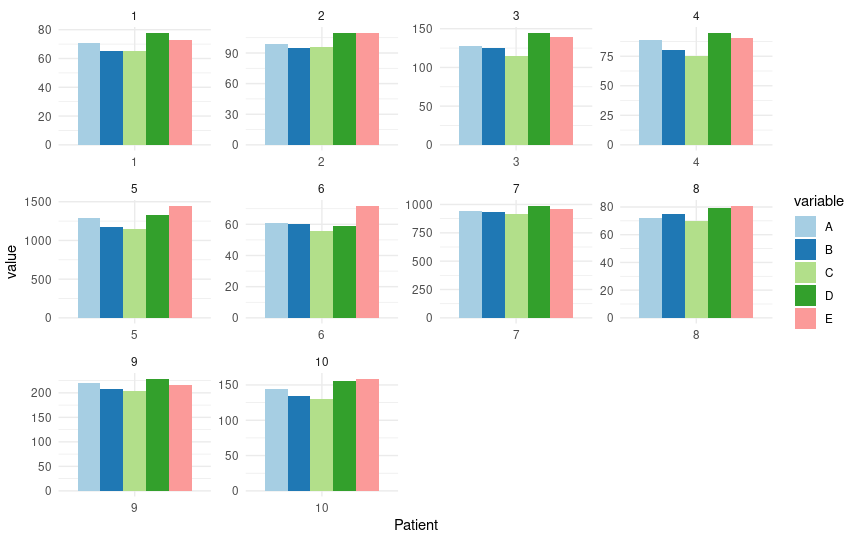
Ten patients did the same test from 5 different companies.
Save the data below as “123.txt”.

Patient	A	B	C	D	E
1	71	65	65	78	73
2	99	95	96	110	110
3	128	125	115	145	139
4	89	80	75	95	90
5	1290	1180	1145	1330	1450
6	61	60	56	59	72
7	945	935	918	990	956
8	72	75	70	79	81
9	220	208	204	229	217
10	145	134	130	155	159

# Read the data
TB <- read.table("123.txt", header=T)
head(TB)

Patient    A    B    C    D    E
1       1   71   65   65   78   73
2       2   99   95   96  110  110
3       3  128  125  115  145  139
4       4   89   80   75   95   90
5       5 1290 1180 1145 1330 1450
6       6   61   60   56   59   72

library(reshape2)
library(ggplot2)

TB$Patient = as.factor(TB$Patient)
TB_g <- melt(TB)

ggplot(TB_g, aes(x= Patient, y = value, fill = variable)) +
  geom_bar(stat="identity", position = "dodge")+
  facet_wrap(~Patient, scale="free") +
  scale_fill_brewer(palette = "Paired")+ theme_minimal()

With normal One-way anova:

one.way <- aov(value~ variable, data = TB_g)
summary(one.way)

TukeyHSD(one.way)

Df  Sum Sq Mean Sq F value Pr(>F)
variable     4   16091    4023   0.021  0.999
Residuals   45 8465019  188112



Tukey multiple comparisons of means
95% family-wise confidence level

Fit: aov(formula = value ~ variable, data = TB_g)

$variable
diff      lwr     upr     p adj
B-A -16.3 -567.441 534.841 0.9999882
C-A -24.6 -575.741 526.541 0.9999393
D-A  15.0 -536.141 566.141 0.9999916
E-A  22.7 -528.441 573.841 0.9999559
C-B  -8.3 -559.441 542.841 0.9999992
D-B  31.3 -519.841 582.441 0.9998416
E-B  39.0 -512.141 590.141 0.9996211
D-C  39.6 -511.541 590.741 0.9995975
E-C  47.3 -503.841 598.441 0.9991880
E-D   7.7 -543.441 558.841 0.9999994

P value is very close to 1 which means that there are no significant difference between 5 companies.
This is worng because it treated all data as independent rather than repeated data

There is how we should deal with the repeated data:

library(tidyverse)
library(rstatix)

res.aov <- anova_test(data = TB_g, dv = value, wid = Patient, within = variable)
res.aov

ANOVA Table (type III tests)

$ANOVA
    Effect DFn DFd     F     p p<.05   ges
1 variable   4  36 2.957 0.033     * 0.002

$`Mauchly's Test for Sphericity`
    Effect        W        p p<.05
1 variable 8.46e-06 2.84e-14     *

$`Sphericity Corrections`
    Effect   GGe     DF[GG] p[GG] p[GG]<.05   HFe     DF[HF] p[HF] p[HF]<.05
1 variable 0.265 1.06, 9.55 0.117           0.271 1.08, 9.76 0.115    

As you can see, the p value from anova result is 0.033 which is signifcant. On the other hand, the reuslt from “Mauchly’s test for Sphericity” is extremely signifcant. But After correction, the p-adjust is not significant. = =

For this data, we using Friedman Test.

The Friedman Test is a non-parametric alternative to the Repeated Measures ANOVA. It is used to determine whether or not there is a statistically significant difference between the means of three or more groups in which the same subjects show up in each group.
Zach from statology; 2020

# p.adjust.method = "holm", "hochberg", "hommel", "bonferroni", "BH", "BY", "fdr", "none"
pwc <- TB_g %>%
      wilcox_test(
        value ~ variable, paired = TRUE,
        p.adjust.method = "bonf"
        )
pwc

# A tibble: 10 × 9
   .y.   group1 group2    n1    n2 statistic     p p.adj p.adj.signif
 *                      
 1 value A      B         10    10      52.5 0.012 0.125 ns          
 2 value A      C         10    10      55   0.002 0.02  *           
 3 value A      D         10    10       1   0.008 0.08  ns          
 4 value A      E         10    10       3   0.014 0.138 ns          
 5 value B      C         10    10      44   0.012 0.125 ns          
 6 value B      D         10    10       1   0.008 0.08  ns          
 7 value B      E         10    10       0   0.002 0.02  *           
 8 value C      D         10    10       0   0.006 0.059 ns          
 9 value C      E         10    10       0   0.002 0.02  *           
10 value D      E         10    10      26   0.722 1     ns   

From the Friedman Test we can see 3 groups are significantly different.
To be notice that this result is slightly different from Prism for some reson. But it is the closed one to it after you choosed “Non parematic and Repeated” for doing ANOVA test.

Anova with rstatix library

Reference: rdrr.io

library(rstatix)

# Load data

TB = data.frame()
for(Chick in unique(ChickWeight$Chick)){
  W = ChickWeight$weight[ChickWeight$Chick==Chick][12] -
  ChickWeight$weight[ChickWeight$Chick==Chick][1]
  Di = ChickWeight$Diet[ChickWeight$Chick==Chick][1]
  TMP = data.frame(Chick = Chick, Diet = Di, Wieght = W)
  TB = rbind(TB, TMP)
}

TB <- na.omit(TB)
summary(TB)

Chick    Diet       Wieght     
1      : 1   1:16   Min.   : 32.0  
2      : 1   2:10   1st Qu.:126.0  
3      : 1   3:10   Median :164.0  
4      : 1   4: 9   Mean   :177.6  
5      : 1          3rd Qu.:225.0  
6      : 1          Max.   :332.0  
(Other):39        

# Compute ANOVA and display the summary
res.anova <- Anova(lm(Wieght ~ Diet, data = TB))
anova_summary(res.anova)

Effect DFn DFd     F     p p<.05   ges
1   Diet   3  41 4.698 0.007     * 0.256

# Compute ANOVA and display the summary
res.anova <- Anova(lm(Wieght ~ Diet, data = TB))
anova_summary(res.anova)