Phylogenetic Tree

What is Phylogenetic Tree

A phylogenetic tree is a diagram representing the evolutionary relationships among species or other entities based on their genetic or physical characteristics. The branches of the tree indicate how these species have evolved from common ancestors. The tree can be rooted, showing the most recent common ancestor, or unrooted, illustrating relationships without a common origin point. Constructed using data like DNA sequences or morphological traits, these trees are essential in studying evolutionary biology, tracking disease evolution, and in conservation efforts. They provide a visual representation of the evolutionary history and connections between different forms of life.
(GPT4)

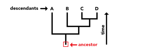
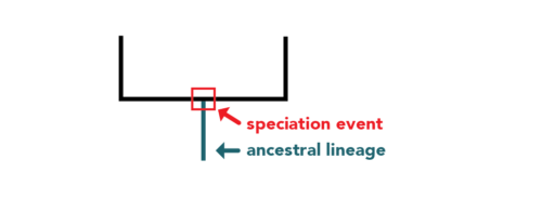
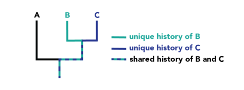
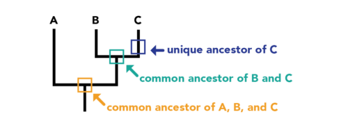
General Ideas of Phylogenetic Tree

Source: Evo 101, Berkeley

Distance Matrix (GPT4)

More related source could be found at academic accelerator

A distance matrix, in general, is a table used to show the distance between elements in a set. In the context of phylogenetics, it represents the genetic distance between various species or sequences.
A distance matrix in phylogenetics is a tool to quantify and visualize the genetic distances between different species or sequences. This matrix forms the basis for constructing phylogenetic trees, which depict the evolutionary relationships and history among the species studied.

1. General Distance Matrix

• This is a square matrix where the elements represent the distances between pairs of objects.
• In the matrix, each row and column represents an object, and each cell in the matrix shows the distance between the two objects.
• The distances can be based on various metrics, depending on the context (e.g., physical distance, similarity in characteristics, etc.).

2. Distance Matrix in Phylogenetics

• In phylogenetics, the distance matrix represents genetic distances between different species or DNA sequences.
• The genetic distance can be based on differences in DNA, RNA, or protein sequences, indicating how much genetic change has occurred between the sequences.
• The distances are often calculated using methods that count the number of differences between sequences (like nucleotide substitutions) or more complex models that account for the rate of evolution and types of mutations.

3. How it Works in Phylogenetics

• Data Collection: First, genetic data (like DNA sequences) from different species or organisms are collected.
• Distance Calculation: Algorithms calculate the genetic distance between each pair of sequences. These calculations can be straightforward (like counting differences) or complex (accounting for evolutionary models).
• Matrix Formation: These distances are then arranged in a matrix format, where each row and column represents a species or sequence, and each cell shows the genetic distance between them.
• Tree Construction: Phylogenetic trees can be constructed using this matrix. Methods like UPGMA (Unweighted Pair Group Method with Arithmetic mean) or neighbor-joining are used to create trees that best reflect the distances in the matrix.
• Analysis: The resulting tree is analyzed to understand evolutionary relationships, like which species are more closely related based on the genetic distances.

© academic accelerator

How to make the sense of the dendrogram?

This graph illustrates the distance matrix and how it gives sense to the phylogenetic tree. According to the tree, the distance between b and c is 1+2=3. Similarly, we can deduce from the tree that the distance between a and d is 4+4+1=9.

Methods for Calculating the Distance Matrix (GPT4)

In phylogenetics, there are several methods to calculate the distance matrix, each with its own approach to measuring genetic distances between sequences. These methods vary in complexity and the types of evolutionary changes they consider. Here are some commonly used methods:

1. Simple Counting Methods

• These involve counting the number of differences (e.g., nucleotide or amino acid substitutions) between each pair of sequences.
• One example is the Hamming distance, which is simply the number of positions at which the corresponding elements (nucleotides or amino acids) are different.

2. Corrected Distance Methods

• These methods account for multiple changes at the same site and unseen changes due to evolutionary processes.
• An example is the Jukes-Cantor model, which corrects for multiple substitutions at the same site by assuming that all changes occur at the same rate.

3. Model-Based Methods

• These use complex models of sequence evolution, accounting for factors like different rates of substitution between different nucleotides or amino acids, transition/transversion bias, and others.
• Examples include the Kimura 2-parameter model and the Tamura-Nei model, which provide more sophisticated ways to estimate genetic distances by incorporating specific evolutionary assumptions.

4. Maximum Likelihood and Bayesian Methods

• These are more computationally intensive methods that use probabilistic models of sequence evolution.
• They estimate the likelihood of observing the data given various possible evolutionary histories and can provide more accurate estimates of genetic distances.

Each of these methods has its own strengths and limitations, and the choice of method often depends on the specifics of the data and the research question. Simple counting methods are straightforward but may underestimate distances, especially when sequences have diverged significantly. Corrected distance and model-based methods provide more accurate estimates by considering the complexities of molecular evolution, but they require more computational resources and deeper understanding of evolutionary models. Maximum likelihood and Bayesian methods are highly accurate but computationally demanding.

In practice, the choice of method is often a balance between the need for accuracy and the availability of computational resources, as well as the evolutionary characteristics of the organisms being studied.

Different Ways to Illustrate the Tree (By GGTREE)

© YuLab@SMU

Something You’d Like to Know About Phylogenetic Trees (Chat4)

When working with phylogenetic trees, there are several key points and common misconceptions to be aware of:

1. Tree Topology Matters More Than Branch Length

The branching pattern (topology) of the tree indicates the evolutionary relationships among the species or genes in the tree. However, unless explicitly stated, the length of the branches might not represent evolutionary time or genetic distance.

2. Branch Points (Nodes) Represent Common Ancestors

Each node where branches diverge represents the most recent common ancestor of the groups branching off from that node.

3. Reading the Tree Correctly

A common misunderstanding is the way to interpret the tree's layout. The tree should be read as a series of branching events, not as a left-to-right progression. The order of groups along the tips of the branches doesn't necessarily indicate any specific type of progression or superiority.

4. Phylogenetic Trees Are Hypothetical

These trees are based on the best available data and the most accurate methods at the time. As new data emerge, the tree might be modified.

5. Rooted vs. Unrooted Trees

Rooted trees have a single ancestral lineage (usually at the base) that serves as a common ancestor for all the entities in the tree. Unrooted trees do not show an ancestral root and are used to illustrate the relationships between different lineages without assuming their descent from a common ancestor.

6. Monophyletic, Paraphyletic, and Polyphyletic Groups

Misunderstanding these terms can lead to confusion. Monophyletic groups include an ancestor and all its descendants, paraphyletic groups include an ancestor and some but not all descendants, and polyphyletic groups are characterized by members that do not share a recent common ancestor in the context of the tree.

7. Convergent Evolution Can Be Misleading

Sometimes, unrelated species may appear closely related due to similar selective pressures rather than shared ancestry, a phenomenon known as convergent evolution.

8. Horizontal Gene Transfer

Especially in bacterial phylogenetics, horizontal gene transfer can complicate the interpretation of evolutionary relationships.

Understanding these points can help in correctly interpreting phylogenetic trees and avoiding common misconceptions. It’s also important to remember that phylogenetics is a constantly evolving field, with new methods and data continually refining our understanding of evolutionary relationships.

Beyond the Distance Matrix (Chat4)

Phylogenetic trees can also be constructed without using a distance matrix. The construction of phylogenetic trees can be broadly categorized into two main approaches: distance-based methods and character-based methods. While distance-based methods do rely on distance matrices, character-based methods do not. Here’s a brief overview of these approaches:

1. Distance-Based Methods: These methods, such as UPGMA (Unweighted Pair Group Method with Arithmetic Mean) and Neighbor-Joining (exp, -QUICKTREE from clustalW), rely on a distance matrix that represents the genetic distance (differences) between pairs of taxa. The matrix is used to construct a tree that represents these distances as accurately as possible.

2. Character-Based Methods: These methods do not use a distance matrix. Instead, they directly analyze the character states (such as DNA, RNA, or protein sequences) of the taxa being studied. There are two primary types of character-based methods:

   • Maximum Parsimony: This method identifies the tree that requires the smallest number of evolutionary changes. It looks for the tree that explains the data with the least amount of complexity, without involving a distance matrix.

   • Maximum Likelihood and Bayesian Methods: These are statistical methods that evaluate different possible phylogenetic trees and choose the tree that is most likely to have produced the observed set of data. These methods are based on explicit models of evolutionary change and do not rely on a pre-calculated distance matrix.

Each method has its advantages and limitations, and the choice of method can depend on the type of data available, the computational resources, and the specific objectives of the study. Character-based methods, especially those involving statistical approaches like Maximum Likelihood and Bayesian Inference, have become increasingly popular due to their ability to incorporate complex models of evolutionary change and handle large datasets effectively.

The Difference Between NJ-Tree and ML-Tree (Chat4)

The popularity and suitability of the Neighbor-Joining (NJ) and Maximum Likelihood (ML) methods for constructing phylogenetic trees depend on the specific requirements and constraints of the research being conducted. Both methods have their advantages and limitations, and their appropriateness can vary based on factors like data complexity, computational resources, and the level of accuracy needed.

Popularity

1. Neighbor-Joining (NJ): Historically, NJ has been very popular, particularly in earlier studies, due to its computational efficiency. It’s well-suited for large datasets where quick, preliminary analyses are needed. NJ’s simplicity and speed made it a go-to method for many researchers, especially before the widespread availability of powerful computational resources.

2. Maximum Likelihood (ML): With the increase in computational power and the development of more sophisticated software, ML has gained substantial popularity, especially in more recent studies. It is often preferred for its ability to provide more accurate and statistically robust trees, especially for complex datasets.

Feature	Neighbor-Joining (NJ)	Maximum Likelihood (ML)
Speed and Efficiency	Fast and efficient, ideal for large datasets and quick analyses.	Slower and computationally intensive, especially with larger datasets.
Accuracy	Less accurate for complex evolutionary models; sensitive to rate variation and sampling errors.	More accurate and statistically robust across a wide range of datasets.
Evolutionary Models	Does not explicitly model evolutionary processes.	Incorporates explicit models of sequence evolution, handling varying rates of evolution better.
Computational Resources	Less demanding, suitable for limited computational resources.	Requires significant computational power for large and complex datasets.
Statistical Support	Limited statistical measures for tree support.	Provides robust statistical measures (like bootstrap values) for tree support.
Use Case	Suitable for preliminary or rapid analyses when computational resources are limited.	Preferred for detailed, accurate phylogenetic analyses where computational resources are available.
Complexity and Understanding	Simpler to understand and use.	Requires a good understanding of evolutionary models and statistical methods.

Conclusion

The choice between NJ and ML largely depends on the specific requirements of your phylogenetic analysis. For preliminary or rapid analyses with large datasets, NJ remains popular due to its speed. However, for in-depth studies where accuracy and model-based statistical rigor are crucial, ML is often considered superior, albeit at the cost of greater computational demand. With ongoing advancements in computational methods and resources, ML is becoming increasingly accessible and popular in phylogenetic studies.

Maximum Likelihood

Maximum Likelihood (ML) is a statistical method used in the construction of phylogenetic trees, which represent the evolutionary relationships among various species or genetic sequences. This method is based on the principle of finding the tree topology (i.e., the arrangement of branches and nodes) that has the highest probability of producing the observed set of genetic data. Here’s a simplified explanation of how it works:

1. Model of Sequence Evolution: ML requires a model of sequence evolution. This model includes parameters such as the rates of different types of mutations (e.g., transitions and transversions in nucleotide sequences), the frequency of each nucleotide or amino acid, and potentially other factors like the rate at which different parts of the sequence evolve. These models attempt to approximate the real biological processes that lead to changes in genetic sequences over time.

2. Tree Topologies: The algorithm considers different possible tree topologies. A topology is a specific arrangement of species or sequences on a tree, indicating how they are related to each other.

3. Calculating Likelihoods: For each tree topology, the likelihood that the observed data (genetic sequences of the species or taxa being studied) would evolve according to the specified model is calculated. This involves complex computations where the algorithm assesses the probability of changes occurring along the branches of the tree to result in the observed sequences at the tree’s tips (leaves).

4. Comparing Trees: The likelihoods of different tree topologies are compared. The tree with the highest likelihood is considered the best estimate of the true evolutionary relationships among the sequences. This is because, under the chosen model, this tree would be the most likely to produce the observed data.

5. Optimization and Searching: Because there are usually an extraordinarily large number of possible tree topologies (increasing exponentially with the number of sequences), it’s impractical to evaluate every possible tree. Therefore, heuristic algorithms are used to search tree space efficiently, focusing on those areas where higher likelihood trees are more likely to be found.

6. Statistical Testing: Often, statistical methods such as bootstrap analysis are used to test the reliability of the tree. This involves resampling the data and recalculating trees to see how often certain groupings appear, providing a measure of confidence in the tree’s branches.

Maximum Likelihood is favored for its statistical rigor and its ability to provide a clear criterion (likelihood) for choosing among trees. However, it is computationally intensive, especially for large datasets, and the results can be sensitive to the choice of the evolutionary model. Despite these challenges, ML remains a popular and powerful method in phylogenetic analysis.

A Simple Practice

In this practice, we generated genetic data for two species and their common ancestor. We then used the Jukes-Cantor model to calculate the likelihood of the observed sequences given a tree topology and a mutation rate. Here’s a summary of the process and results:

• Generated Data: We created random genetic sequences for a common ancestor and two descendant species.
• Jukes-Cantor Model: This model was used to estimate the likelihood of one sequence evolving into another under a uniform mutation rate.
• Initial Likelihood Calculation: For the given tree topology (where the common ancestor is the parent of both species), we calculated the likelihood of this tree using a mutation rate of 0.1. The likelihood was found to be approximately 20.46.
• Optimization: We used an optimization algorithm to find the mutation rate that maximizes the likelihood of the observed data given the tree structure. The optimal mutation rate was found to be 1.0.
• Optimized Likelihood: Recalculating the likelihood with the optimized mutation rate, we obtained an improved likelihood of approximately 7.05.

This demonstration shows how Maximum Likelihood is used in phylogenetics to find the most likely tree structure and parameters (like mutation rate) that explain the observed genetic data. In real-world scenarios, the data and models are much more complex, and the computations are more intensive, but the underlying principles remain the same. ​

# Corrected implementation for demonstrating Maximum Likelihood in phylogenetics

# Generate a simple example dataset with direct ancestor-descendant relationships
np.random.seed(0)
# Assume we have two species and their common ancestor
data = {
    "Common_Ancestor": np.random.choice(['A', 'T', 'G', 'C'], 10),
    "Species_A": np.random.choice(['A', 'T', 'G', 'C'], 10),
    "Species_B": np.random.choice(['A', 'T', 'G', 'C'], 10)
}
df = pd.DataFrame(data)
print("Generated Genetic Data:\n", df)

# Define a simple model of sequence evolution
def jukes_cantor_model(seq1, seq2, mu):
    """
    Jukes-Cantor model to calculate the likelihood of seq2 evolving from seq1
    under a uniform mutation rate mu.
    """
    diff = sum(c1 != c2 for c1, c2 in zip(seq1, seq2))
    same = len(seq1) - diff
    p_diff = 3/4 * (1 - np.exp(-4/3 * mu))
    p_same = 1/4 + 1/4 * np.exp(-4/3 * mu)

    likelihood = (p_diff ** diff) * (p_same ** same)
    return likelihood

# Function to calculate the likelihood of a tree given the data
def tree_likelihood(tree, data, mu):
    """
    Calculate the likelihood of a given tree topology.
    The tree is represented as a dictionary where keys are nodes and values are the sequences.
    """
    likelihood = 1.0
    for parent, child in tree.items():
        parent_seq = data[parent]
        child_seq = data[child]
        likelihood *= jukes_cantor_model(parent_seq, child_seq, mu)
    return -log(likelihood)  # negative log-likelihood for optimization

# Example tree topology (parent: child)
tree_example = {
    "Common_Ancestor": "Species_A",
    "Common_Ancestor": "Species_B",
}

# Assume a mutation rate (mu)
mu = 0.1

# Calculate the likelihood of this tree
likelihood = tree_likelihood(tree_example, df, mu)
print("\nLikelihood of the tree:", likelihood)

# Now we will use optimization to find the mutation rate that maximizes the likelihood
def optimize_mu(mu, tree, data):
    return tree_likelihood(tree, data, mu)

result = minimize(optimize_mu, x0=mu, args=(tree_example, df), bounds=[(0.001, 1)])
optimal_mu = result.x[0]
print("\nOptimal mutation rate:", optimal_mu)

# Recalculate the likelihood with the optimized mutation rate
optimized_likelihood = tree_likelihood(tree_example, df, optimal_mu)
print("\nOptimized likelihood of the tree:", optimized_likelihood)

Generated Genetic Data:
   Common_Ancestor Species_A Species_B
0               A         T         G
1               C         G         C
2               T         A         C
3               A         C         G
4               C         G         A
5               C         A         T
6               C         A         T
7               C         A         T
8               T         G         T
9               C         T         A

Likelihood of the tree: 20.463275567320334
Optimal mutation rate: 1.0
Optimized likelihood of the tree: 7.05394379820434

Things You’d Like to Know

1. Pairwise Comparisons: In the ML approach, the focus is not typically on pairwise comparisons between sequences (as it is in methods like distance matrix or neighbor-joining). Instead, ML evaluates the likelihood of entire tree topologies. It looks at how likely it is for a given tree structure, with its branching pattern and lengths, to have produced the observed set of genetic sequences under a specific evolutionary model.

2. Likelihood Calculations: For each possible tree topology, ML calculates the likelihood that the proposed tree would result in the observed data (e.g., DNA, RNA, or protein sequences). This calculation involves estimating the probability of changes in the sequences along each branch of the tree. The likelihood depends on both the tree topology (how the branches are arranged) and the model parameters (like mutation rates).

3. Optimization: The goal is to find the tree topology (and associated model parameters) that maximizes the likelihood. Due to the vast number of possible trees, especially with larger datasets, heuristic search algorithms are used to navigate the space of possible trees efficiently.

4. Likelihood Matrix: Unlike methods that rely on a distance matrix, ML doesn’t typically produce a matrix of pairwise likelihoods. Instead, it directly evaluates the likelihood of entire tree topologies.

5. Resulting Tree: The end result of an ML analysis is a single tree (or sometimes a set of trees) that has the highest likelihood given the data and the chosen model. This tree represents the estimated evolutionary relationships among the sequences.

6. Dendrogram/Phylogenetic Tree: The final output is a phylogenetic tree (often visualized as a dendrogram) that represents the hypothesized evolutionary relationships among the species or sequences analyzed. This tree is based on the topology that provided the highest likelihood.

In summary, while ML involves complex calculations involving the entire tree, it doesn’t use a pairwise likelihood matrix in the same way that distance-based methods use a distance matrix. The primary focus of ML is on evaluating and comparing the likelihoods of different tree topologies to find the one that best explains the observed data under a given evolutionary model.